Correlation-Based Clustering: Spectral Clustering Methods
Clustering consists in trying to identify groups of “similar behavior”1 - called clusters - from a dataset, according to some chosen characteristics.
An example of such a characteristic in finance is the correlation coefficient between two time series of asset returns, whose usage to partition a universe of assets into groups of “close” and “distant” assets thanks to a hierarchical clustering method was originally2 proposed in Mantegna3.
In this blog post, I will describe two correlation-based clustering methods belonging to the family of spectral clustering methods: the Blockbuster method introduced in Brownlees et al.4 and the SPONGE method introduced in Cucuringu et al.5.
As examples of usage, I will discuss 1) how to automatically group U.S. stocks together without relying on external information like industry classification and 2) how to identify risk-on and risk-off assets within a U.S. centric universe of assets.
Mathematical preliminaries
Let $x_1$, …, $x_n$ be $n$ points6 in $\mathbb{R}^m, m \geq 1$ to be partitioned into $k \geq 2$ subsets.
Spectral clustering
Spectral clustering, like other approaches to clustering - geometric approaches such as $k$-means , density-based approaches such as DBSCAN… - initially relies on pairwise similarities $s(x_i, x_j)$ between points $i,j=1..n$ with $s$ some similarity function which is symmetric and non-negative1.
Once the corresponding similarity matrix $S_{ij} = s(x_i, x_j)$, $i,j=1…n$, has been computed, a spectral clustering method then usually follows a three-step process:
-
Compute an affinity matrix $A \in \mathbb{R}^{n \times n}$ from the similarity matrix $S$
The affinity matrix $A$ corresponds to the adjacency matrix of an underlying graph whose vertices represent the points $x_1$, …, $x_n$ and whose edges model the local7 neighborhood relationships between the data points1.
-
Compute a matrix $L \in \mathbb{R}^{n \times n}$ derived from the affinity matrix $A$
Due to the relationship between spectral clustering and graph theory1, the matrix $L$ is typically called a Laplacian matrix.
-
Compute a matrix $Y \in \mathbb{R}^{n \times k}$ derived from the eigenvectors corresponding to the $k$ smallest (or sometimes largest) eigenvalues of the matrix $L$ and cluster its $n$ rows $y_1$, …, $y_n$ using the $k$-means algorihm
The result of that clustering represents the desired clustering of the original $n$ points $x_1$, …, $x_n$.
It should be emphasized that there is nothing principled about using the $k$-means algorithm in this step1, c.f. for example Huang et al.8 in which spectral rotations are used instead of $k$-means, but one can argue that at least the Euclidean distance between the [rows of the matrix $Y$] is a meaningful quantity to look at1.
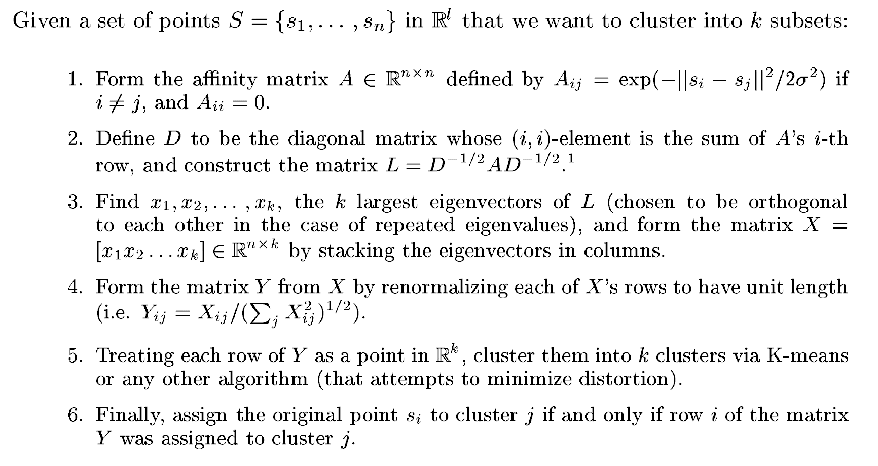
The Ng-Jordan-Weiss spectral clustering method
Different ways of computing the affinity matrix $A$, the Laplacian matrix $L$ or the matrix $Y$ lead to different spectral clustering methods9.
One popular spectral clustering method is the Ng-Jordan-Weiss (NJW) method10, detailed in Figure 1 taken from Ng et al.10 where $\sigma^2$ is a scaling parameter that controls how rapidly the affinity $A_{ij}$ falls off with the distance between $s_i$ and $s_j$10.
Rationale behind spectral clustering
At first sight, [spectral clustering] seem to make little sense. Since we run $k$-means [on points $y_1$, …, $y_n$], why not just apply $k$-means directly to the [original points $x_1$, …, $x_n$]10?
A visual justification of spectral clustering is provided in Figure 2 adpated from Ng et al.10, which displays data points in $\mathbb{R}^2$ forming two circles (e) and their associated spectral representation in $\mathbb{R}^2$ using the NJW spectral clustering method (h).
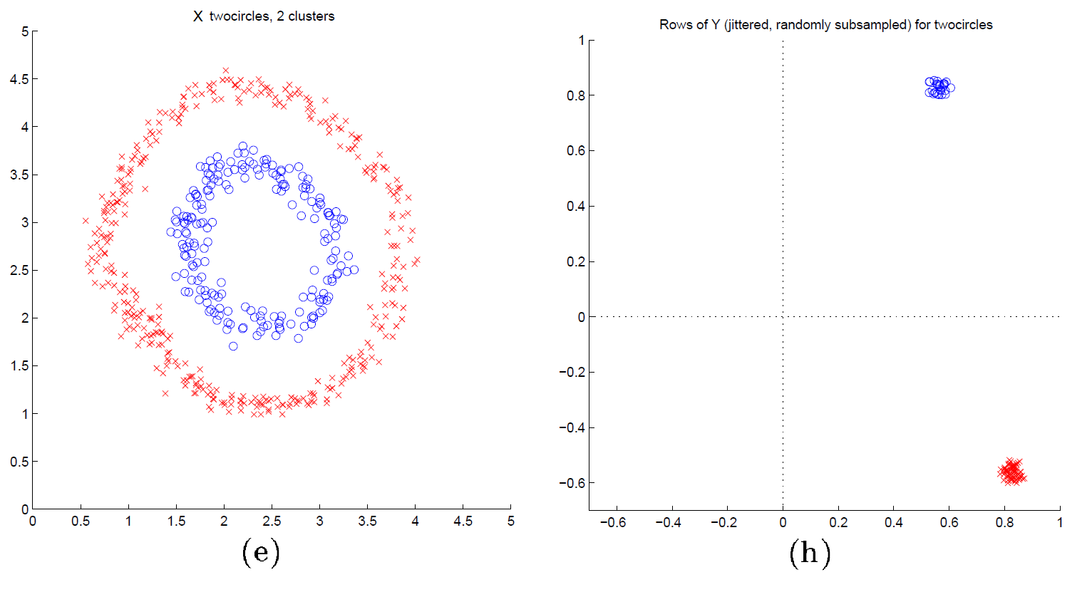
On Figure 2, it is clearly visible that the transformed data points (h) form two well-separated convex clusters in the spectral plane, which is the ideal situation for the $k$-means algorithm.
More generally11, it can be demonstrated that the change of representation from the original data points $x_1$, …, $x_n$ to the embedded data points $y_1$, …, $y_n$ enhances the cluster-properties in the data, so that clusters can be trivially detected [by the $k$-means clustering algorithm] in the new representation1.
Correlation-based spectral clustering
Let $x_1$, …, $x_n$ be $n$ variables whose pairwise correlations12 $\rho_{ij}$, $i,j=1…n$, have been assembled in a correlation matrix $C \in \mathbb{R}^{n \times n}$.
Because correlation is a measure of dependency, a legitimate question is whether it is possible to use spectral clustering to partition these variables w.r.t. their correlations? Ideally, we would like to have highly correlated variables grouped together in the same clusters, with low or even negative correlations between the clusters themselves.
Problem is, as noted in Mantegna3, the correlation coefficient of a pair of [variables] cannot be used as a distance [or as a similarity] between the two [variables] because it does not fulfill the three axioms that define a metric3, which a priori excludes its direct usage in a similarity matrix or in an affinity matrix.
That being said, a13 metric14 can be defined using as distance a function of the correlation coefficient3 - like the distance $ d_{ij} = \sqrt{ 2 \left( 1 - \rho_{ij} \right) } $ -, which allows to indirectly use any spectral clustering method15 with correlations.
But what if we insist to work directly with correlations? In this case, a couple of specific spectral clustering methods have been developped, among which:
- The Blockbuster spectral clustering method of Brownlees et al.4
- The SPONGE spectral clustering method of Cucuringu et al.5
The Blockbuster spectral clustering method
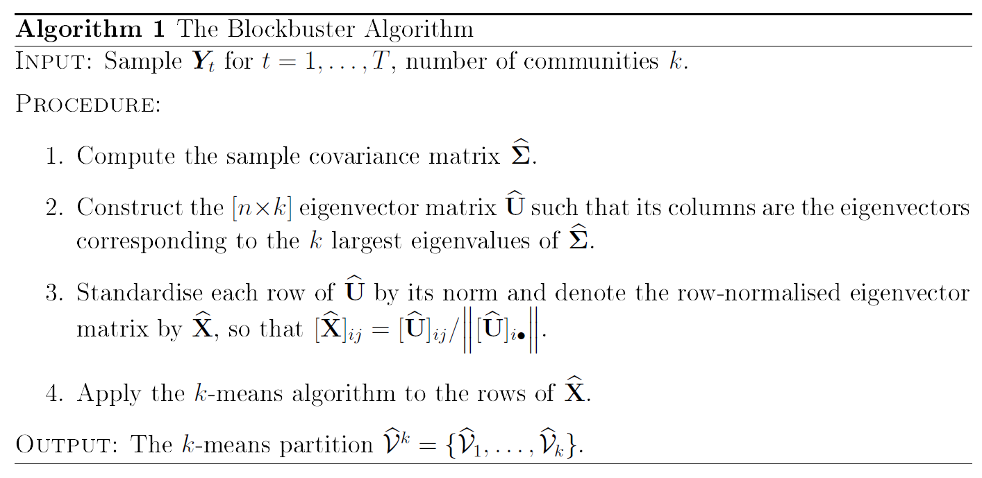
Brownlees et al.4 introduces a network model16 under which large panels of time series are partitioned into latent groups such that correlation is higher within groups than between them4 and proposes an algorithm relying on the eigenvectors of the sample covariance matrix17 $\Sigma \in \mathbb{R}^{n \times n}$ to detect these groups.
As can be seen in Figure 3 taken from Brownlees et al.4, this algorithm - called Blockbuster - is surprisingly very close to the NJW spectral clustering method.
Brownlees et al.4 establishes that the Blockbuster algorithm consistently detects the [groups] when the number of observations $T$ and the dimension of the panel $n$ are sufficiently18 large4, as long as a couple of assumptions are satisfied, like:
- $T \geq n$, with the more fat-tailed and dependent the data are, the larger $T$ has to be4
- The precision matrix $\Sigma^{-1}$ exists and contains only non-positive entries (or its fraction of positive entries is appropriately controlled19)
An important feature of the Blockbuster algorithm is that it allows one to detect the [groups] without estimating the network structure of the data4. In other words, while the Blockbuster algorithm is a spectral clustering method, nowhere is an affinity matrix computed!
The black magic at work here is that the underlying network model of Brownlees et al.4 additionally assumes that the (symmetric normalized) Laplacian matrix $L$ is a function of the precision matrix $\Sigma^{-1}$ through
\[L = \frac{\sigma^2}{\phi} \Sigma^{-1} - \frac{1}{\phi} I_n\], where:
- $\sigma^2$ is a network variance parameter that does not influence the detection of the groups
- $\phi$ is a network dependence parameter that does not influence the detection of the groups
- $I_n \in \mathbb{R}^{n \times n}$ is the identity matrix of order $n$
This formula clarifies the otherwise mysterious connection20 between the Blockbuster algorithm and the NJW method.
The SPONGE spectral clustering method
Cucuringu et al.5 extends the spectral clustering framework described in the previous section to the case of a signed affinity matrix $A$ whose underlying complete weighted graph represents the variables $x_1$, …, $x_n$ and their pairwise correlations.
Figure 4 taken from Jin et al.21 illustrates the idea of Cucuringu et al.5, which is to minimize the number of violations in the constructed partition, with a violation, as in this figure, is when there are negative edges in a cluster and positive edges across clusters21.
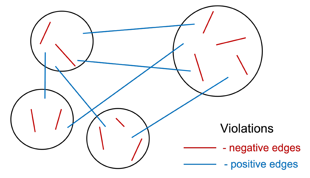
More formally, Cucuringu et al.5 proposes a three-step algorithm22 - called SPONGE (Signed Positive Over Negative Generalized Eigenproblem) - that aims to find a partition [of the underlying graph] into k clusters such that most edges within clusters are positive, and most edges across clusters are negative5:
- Decompose the adjacency matrix as $A = A^+ - A^-$, with
- $A^+ \in \mathbb{R}^{n \times n}$, with $A^+_{ij} = A_{ij}$ if $A_{ij} \geq 0$ and $A^+_{ij} = 0$ if $A_{ij} < 0$
- $A^- \in \mathbb{R}^{n \times n}$, with $A^-_{ij} = A_{ij}$ if $A_{ij} \leq 0$ and $A^-_{ij} = 0$ if $A_{ij} > 0$
- Compute the (unnormalized) positive and negative Laplacian matrices $L^+$ and $L^-$, with
- $L^+ \in \mathbb{R}^{n \times n}$, with $L^+ = D^+ - A^+$ and $D^+ \in \mathbb{R}^{n \times n}$ a diagonal matrix satisfying $D^+_{ii} = \sum_{j=1}^n A^+_{ij}$
- $L^- \in \mathbb{R}^{n \times n}$, with $L^- = D^- - A^-$ and $D^- \in \mathbb{R}^{n \times n}$ a diagonal matrix satisfying $D^-_{ii} = \sum_{j=1}^n A^-_{ij}$
- Compute the matrix $Y \in \mathbb{R}^{n \times k}$ made of the eigenvectors corresponding to the $k$ smallest eigenvalues of the matrix $\left( L^- + \tau^+ D^+ \right)^{-1/2} \left( L^+ + \tau^- D^- \right) \left( L^- + \tau^+ D^+ \right)^{-1/2}$, where $\tau^+ > 0$ and $\tau^- > 0$ are regularization parameters23, and cluster its $n$ rows using the $k$-means algorihm
Cucuringu et al.5 establishes the consistency24 of the SPONGE algorithm in the case of $k = 2$ equally-sized clusters, provided $\tau^-$ is sufficiently small25 compared to $\tau^+$5 and the number of variables $n$ is sufficiently large26 for a clustering to be recoverable5.
In subsequent work, Cucuringu et al.27 establish the consistency24 of a variant of the SPONGE algorithm - called symmetric28 SPONGE - in the case of $k \geq 2$ unequal-sized clusters when $n$ is large enough27.
How to choose the number of clusters in correlation-based spectral clustering?
Choosing the number $k$ of clusters is a general problem for all clustering algorithms, and a variety of more or less successful methods have been devised for this problem1.
Correlation-based spectral clustering being 1) a clustering method 2) based on the spectrum of a matrix derived from 3) a correlation matrix, there are at least three families of methods which can be used to determine the “optimal” number of clusters:
- Generic methods
- Specific methods taylored to spectral clustering
- Specific methods taylored to correlation-based clustering or to correlation-based factor analysis
However, even if it is mathematically satisfying to find such an optimal number, it is important to keep in mind that just because we find an [optimal] partition […] does not preclude the possibility of other good partitions29.
Indeed, as Wang and Rohe29 puts it:
We must disabuse ourselves of the notion of “the correct partition”. Instead, there are several “reasonable partitions” some of these clusterings might be consistent with one another (as might be imagined in a hierarchical clustering), others might not be consistent.
Generic methods
Any black box method to select an optimal number of clusters in a clustering algorithm - like the silhouette index30 or the gap statistic31 - can be used in correlation-based spectral clustering.
On an opinionated note, though, the the elbow criterion should not be used, for reasons detailled in Schubert32.
Specific methods taylored to spectral clustering
In the context of spectral clustering, several specific methods for determining the optimal number of clusters have been proposed.
The most well-known of these methods is the eigengap heuristic1, whose aim is to choose the number $k$ such that all eigenvalues $\lambda_1$,…,$\lambda_k$ [of the Laplacian matrix] are very small, but $\lambda_{k+1}$ is relatively large1. In practice, this method works well if the clusters in the data are very well pronounced1. Nevertheless, the more noisy or overlapping the clusters are, the less effective is this heuristic1, which is obviously a problem for financial applications33. Furthermore, just because there is a gap, it doesn’t mean that the rest of the eigenvectors are noise29.
Another popular method is the method used in the self-tuning spectral clustering algorithm of Zelnik-Manor and Perona34, which selects the optimal number of clusters as the number allowing to “best” align the (rows of the) eigenvectors of the Laplacian matrix with the vectors of the canonical basis of $\mathbb{R}^{k}$.
Specific methods taylored to correlation-based clustering or to correlation-based factor analysis
Correlation-based clustering, whether spectral or not, revolves around a very special object - a correlation matrix -, whose properties can be used to find the optimal number of clusters.
Random matrix theory-based methods
From random matrix theory, the distribution of the eigenvalues of a large random correlation matrix follows a particular distribution - called the Marchenko-Pastur distribution - independent35 of the underlying observations.
That distribution involves a threshold $\lambda_{+} \geq 0$ beyond which it is not expected to find any eigenvalue in a random correlation matrix.
Laloux et al.36 uses this threshold to define a correlation matrix denoising procedure called the eigenvalues clipping method, c.f. a previous blog post.
In the context at hand, Jin et al.21 proposes to determine the optimal number of clusters as the number of eigenvalues of the correlation matrix that exceed [this threshold], which are the eigenvalues associated with dominant factors or patterns in the [original data]21.
To illustrate this method, Figure 5, taken from Laloux et al.36, depicts two different Marchenko-Pastur distributions fitted to a correlation matrix of37 406 stocks belonging to the S&P 500 index.
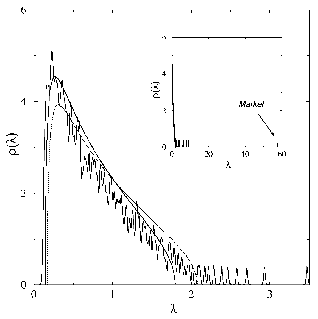
From this figure, the number of clusters corresponding to the method of Jin et al.21 when applied to the dotted Marchenko-Pastur distribution would be around 15.
Non-linear shrinkage-based methods
De Nard38 notes that non-linear shrinkage [of the sample covariance matrix] pushes the sample eigenvalues toward their closest and most numerous neighbors, thus toward (local) cluster38.
As a consequence, it should be possible to use the information from non-linear shrinkage — the number of jumps in the shrunk eigenvalues — or directly the distribution of the sample eigenvalues — the number of sample eigenvalue clusters — to obtain38 the optimal number of clusters.
This method is illustrated in Figure 6 taken from de Nard38, on which 2 clusters are visible.
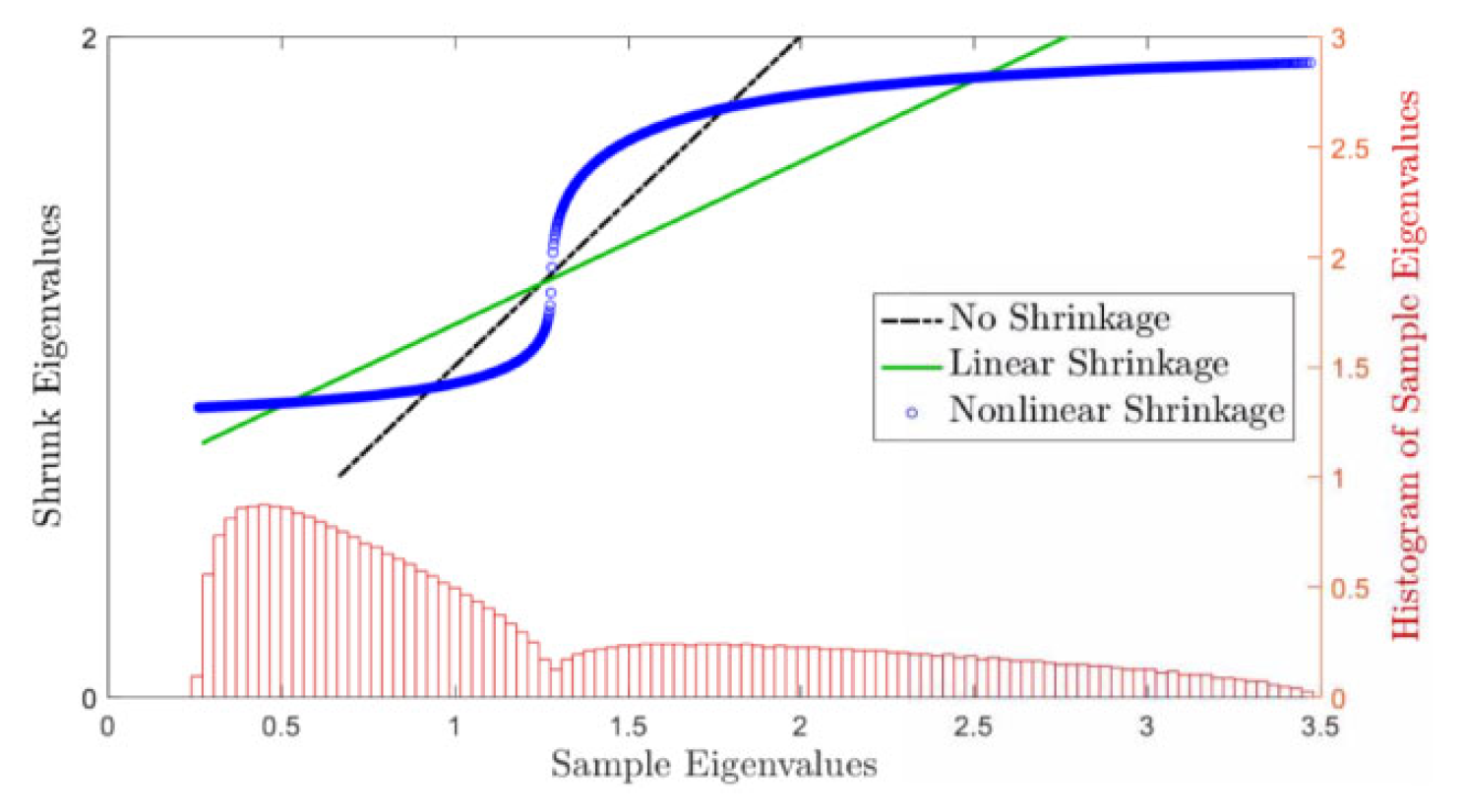
From a practical perspective, de Nard38 suggests to use 1D KDE clustering in order to determine the number of sample eigenvalue clusters.
Factor analysis-based methods
Although the ultimate goal of cluster analysis and factor analysis is different, the underlying logic of both techniques is dimension reduction (i.e., summarizing information on multiple variables into just a few variables)39.
Based on this similarity, de Nard38 discusses the eigenvalue ratio estimator40 of Ahn and Horenstein40 that consists in maximizing the ratio of two adjacent eigenvalues [of the sample correlation matrix41] to determine the number of factors (here clusters)38 in economic or financial data40.
Unfortunately, the eigenvalue ratio estimator often cannot identify any cluster [in a large universe of U.S. stocks] and sets $k = 1$38, which corresponds to the situation described in Ahn and Horenstein40 where one factor [- here, the market factor -] has extremely strong explanatory power for response variables40. In such a situation, the growth ratio estimator40 of Ahn and Horenstein40 - this time maximizing the ratio of the logarithmic growth rate of two consecutive eigenvalues to determine the number of factors - should be used instead, because it empirically appears to be able to mitigate the effect of the dominant factor40.
Yet another estimator of the number of common factors is the adjusted correlation thresholding estimator42 of Fan et al.42, which determines the number of common factors as the number of eigenvalues greater than 1 of the population correlation matrix […], taking into account the sampling variabilities and biases of top sample eigenvalues42.
Implementation in Portfolio Optimizer
Portfolio Optimizer implements correlation-based spectral clustering through the endpoint /assets/clustering/spectral/correlation-based.
This endpoint supports three different methods:
- The Blockbuster spectral clustering method
- The SPONGE spectral clustering method
- The symmetric SPONGE spectral clustering method (default)
As for the number of clusters to use, this endpoint supports:
- A manually-defined number of clusters
- An automatically-determined number of clusters, computed through a proprietary variation of Horn’s parallel analysis method43 (default)
As a side note, Horn’s parallel analysis method seems to be little known in finance, but numerous studies [in psychology] have consistently shown that [it] is the most nearly accurate methodology for determining the number of factors to retain in an exploratory factor analysis44.
Examples of usage
Automated clustering of U.S. stocks
De Nard38 and Jin et al.21 both study the automated clustering of a dynamic universe of U.S. stocks through correlation-based45 spectral clustering:
-
De Nard38, in the context of covariance matrix shrinkage
It uses the Blockbuster method, together with a 1D KDE clustering method to automatically determine the number of clusters.
-
Jin et al.21, in the context of the construction of statistical arbitrage portfolios
It uses the SPONGE and SPONGE symmetric methods, together with a Marchenko-Pastur distribution-based method46 to automatically determine the number of clusters.
An important remark at this point.
When clustering stocks, it is possible to rely on what de Nard38 calls external information38, for example industry classifications like:
Nevertheless, such an external information may fail to create (a valid number of) homogeneous groups38.
In the words of de Nard38:
For example, if we cluster the covariance matrix into groups of financial and nonfinancial firms, arguably, there will be some nonfinancial firm(s) that has (have) some stock characteristics more similar to the financial stocks as to the non-financial stocks and is (are) therefore misclassified. Especially in large dimension one would expect a few of such misclassifications in both directions. To overcome this misclassification problem and to really create homogeneous groups, [a data-driven procedure should be used instead].
Results of de Nard38 and Jin et al.21 are the following:
- Within a universe of 500 stocks over the period January 1998 to December 2017, de Nard38 finds that the number of clusters is limited to only 1 or 2 about 75% of the time.
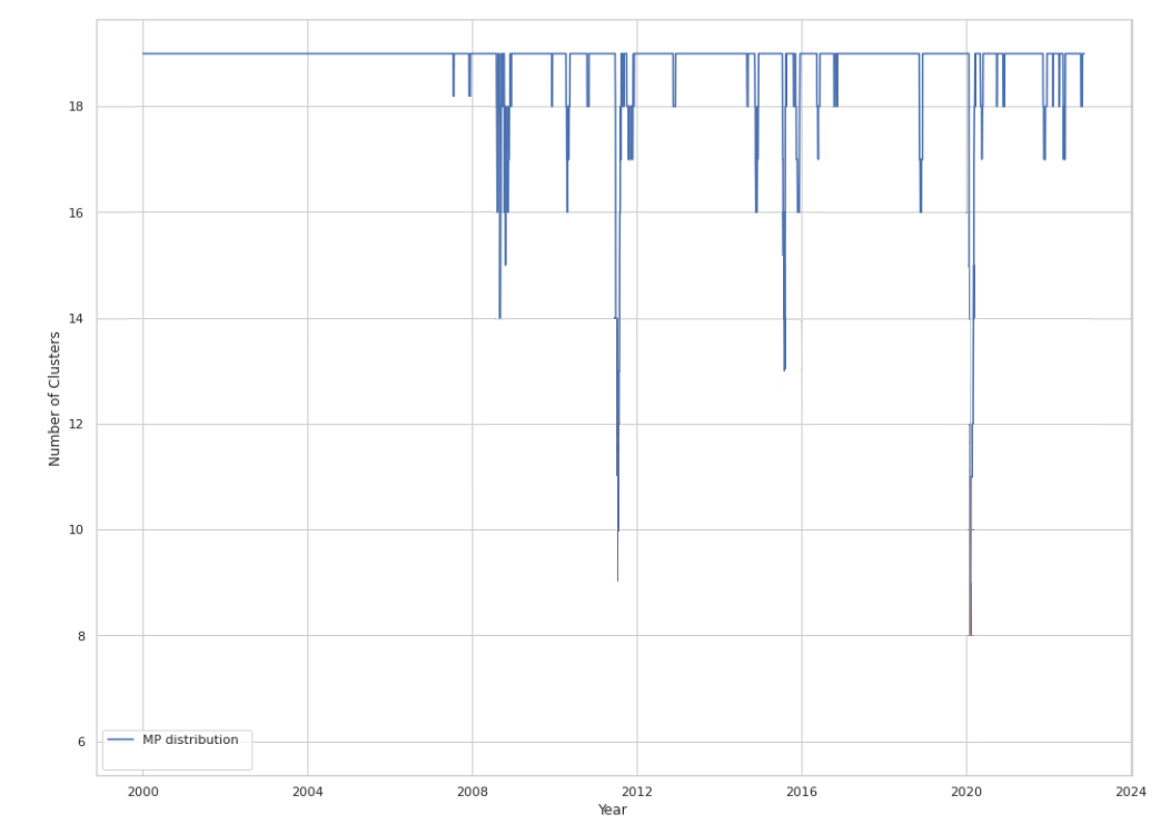
- Within a universe of ~600 stocks over the period January 2000 to December 2022, Jin et al.21 finds that the number of clusters is relatively stable around 19, even though it tends to drop during financial hardships of the United States21 down to a minimum of 8, as displayed in Figure 7 adapted from Jin et al.21.
These diverging results on closely related data sets show that different methods to determine the number of clusters to use in clustering analysis might be completely at odds with one another47.
But these results also show that the “optimal” number of clusters - whatever it is - is not constant over time and that methods that dynamically determine [it] can capture changes in market dynamics, especially when there is significant downside risks in the market21. Incidentally, this is another argument in favor of not relying on (slowly evolving) external information to determine the number of clusters to use.
Identification of risk-on/risk-off assets in a U.S.-centric universe of assets
In April 2025, “risk on/risk off” has been making the headlines as a phrase describing investment and asset price behavior48.
Lee48 summarizes the underlying meaning as follows48:
[…] risk on/risk off generally refers to an investment environment in which asset price behavior is largely driven by how risk appetite advances or retreats over time, usually in a synchronized way at a faster than normal pace across global regions and assets.
And describes it in more details as follows48:
Depending on the environment, investors tend to buy or sell risky assets across the board, paying less attention to the unique characteristics of these assets. Volatilities and, most noticeably, correlations of assets that are perceived as risky will jump, particularly during risk-off periods, inspiring comments such as “correlations go to one” during a crisis. Assets, such as U.S. Treasury bonds, and currencies, such as the Japanese yen, tend to move in the opposite direction of risky assets and are generally perceived as the safer assets to hold in the event of a flight to safety.
In this sub-section, I propose to study the capability of correlation-based spectral clustering to identify risk-on/risk-off assets in a U.S.-centric universe of assets.
For this:
- I will use as a universe of assets 13 ETFs representative49 of misc. asset classes:
- U.S. stocks (SPY ETF)
- European stocks (EZU ETF)
- Japanese stocks (EWJ ETF)
- Emerging markets stocks (EEM ETF)
- U.S. REITs (VNQ ETF)
- International REITs (RWX ETF)
- Cash (SHY ETF)
- U.S. 7-10 year Treasuries (IEF ETF)
- U.S. 20+ year Treasuries (TLT ETF)
- U.S. Investment Grade Corporate Bonds(LQD ETF)
- U.S. High Yield Corporate Bonds (HYG ETF)
- Commodities (DBC ETF)
- Gold (GLD ETF)
-
I will compute the correlation matrix of the daily returns of these assets over the period 1st April 2025 - 30th April 202550
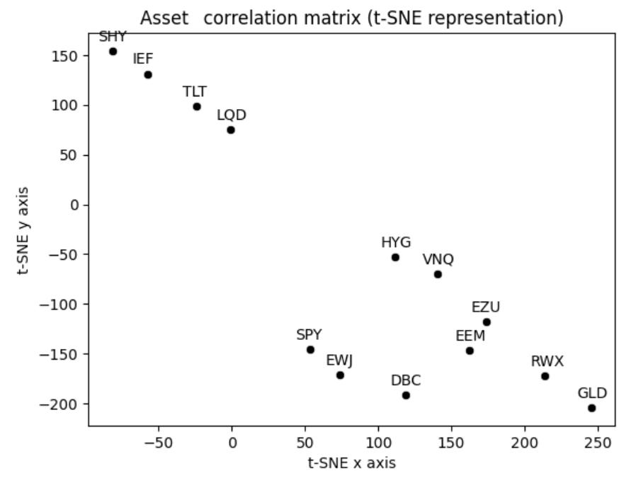
Figure 8 displays that correlation matrix using a planar t-SNE representation of its rows, considered as points in $\mathbb{R}^{13}$.
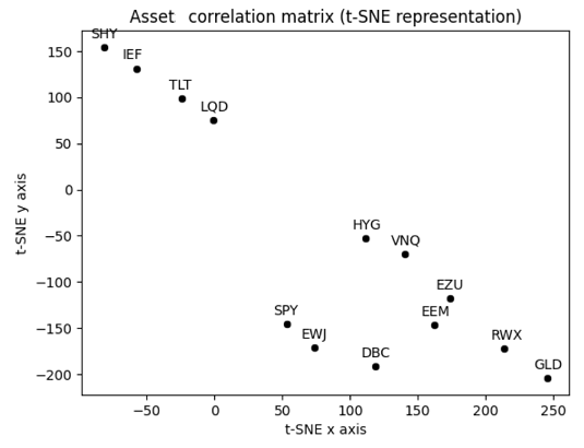
Figure 8. t-SNE representation of the asset correlation matrix, April 2025. To be noted that the t-SNE representation of Figure 8 is a bit misleading in the context of spectral clustering, because spectral clustering does not operate in the t-SNE plane. Still, it is an helpful representation to give a sense of asset “closeness” in terms of correlations.
- I will cluster these assets using the symmetric SPONGE spectral clustering method with $k = 2$ and $k = 3$ clusters, the rationale being that:
- All the assets clustered together with Cash should correspond to risk-off assets ($k = 2,3$)
- All the assets clustered together with U.S. stocks should correspond to risk-on assets ($k = 2,3$)
- All the assets clustered in the remaining cluster should correspond to a another category to be determined ($k = 3$ only)
Figures 9 and 10 show the resulting clusterings.
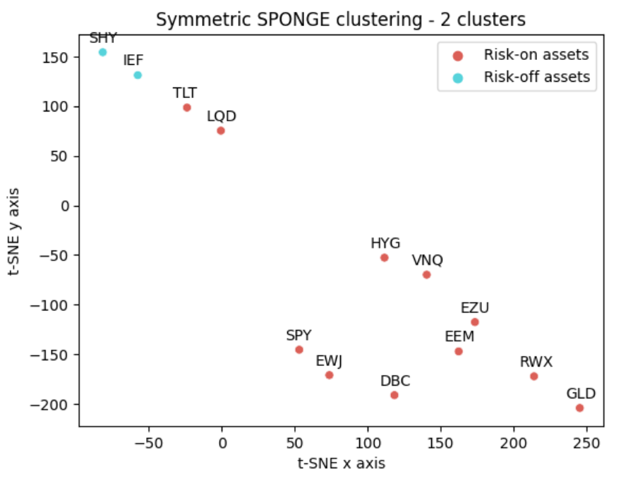
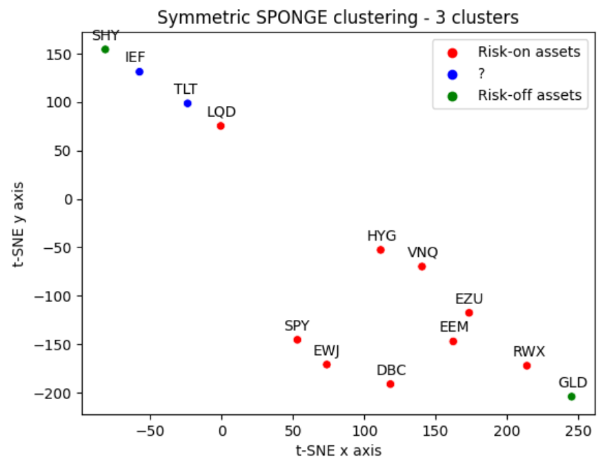
From these figures, and over the considered period:
- Intermediate-term U.S. Treasuries is found to be a risk-off asset when $k = 2$
- Gold is found to be a risk-off asset when $k = 3$, with Intermediate-term and Long-term U.S. Treasuries now moved into their own cluster
The evolution of the classification of Gold as a risk-off asset is particularly interesting51 and also serves to illustrate one of the limitations of the t-SNE representation of the asset correlation matrix.
Indeed, from that representation, it makes no sense that Cash and Gold could belong to the same cluster since they are complete opposites in the t-SNE plane! But in reality, if the t-SNE plane is diagonally “folded”, Cash and Gold truly are close neighbors…
Conclusion
This (abruptly?) concludes this already too long overview of correlation-based spectral clustering.
Waiting for the next blog post on correlation-based clustering, feel free to connect with me on LinkedIn or to follow me on Twitter.
–
-
See von Luxburg, U. A tutorial on spectral clustering. Stat Comput 17, 395–416 (2007). ↩ ↩2 ↩3 ↩4 ↩5 ↩6 ↩7 ↩8 ↩9 ↩10 ↩11 ↩12
-
See R. N. Mantegna, H. E. Stanley, Introduction to econophysics: correlations and complexity in finance, Cambridge university press, 1999. ↩
-
See Mantegna, R.N. Hierarchical structure in financial markets. Eur. Phys. J. B 11, 193–197 (1999). ↩ ↩2 ↩3 ↩4
-
See Brownlees, C., Guðmundsson, G. S., & Lugosi, G. (2020). Community Detection in Partial Correlation Network Models. Journal of Business & Economic Statistics, 40(1), 216–226. ↩ ↩2 ↩3 ↩4 ↩5 ↩6 ↩7 ↩8 ↩9 ↩10
-
See Mihai Cucuringu, Peter Davies, Aldo Glielmo, and Hemant Tyagi. SPONGE: A generalized eigenproblem for clustering signed networks. In Artificial Intelligence and Statistics, volume 89 of Proceedings of Machine Learning Research, pages 1088–1098. PMLR, 2019. ↩ ↩2 ↩3 ↩4 ↩5 ↩6 ↩7 ↩8 ↩9
-
$x_1, …, x_n$ can be more general “objects”, as long as a distance between these objects is defined. ↩
-
As opposed to their global relationships that already available from the similarity matrix $S$. ↩
-
See Jin Huang, Feiping Nie, and Heng Huang. 2013. Spectral rotation versus K-means in spectral clustering. In Proceedings of the Twenty-Seventh AAAI Conference on Artificial Intelligence (AAAI’13). AAAI Press, 431–437. ↩
-
The similarity function $s$ is also very important in spectral clustering, although ultimately, the choice of the similarity function depends on the domain the data comes from, and no general advice can be given1. ↩
-
See Andrew Y. Ng, Michael I. Jordan, and Yair Weiss. 2001. On spectral clustering: analysis and an algorithm. In Proceedings of the 15th International Conference on Neural Information Processing Systems: Natural and Synthetic (NIPS’01). MIT Press, Cambridge, MA, USA, 849–856. ↩ ↩2 ↩3 ↩4 ↩5
-
Thanks to the properties of the Laplacian matrix $L$. ↩
-
Typically the Pearson correlation, but other measures like the Spearman correlation or the Gerber correlation can also be used as long as the resulting correlation matrix $C$ is a valid correlation matrix. ↩
-
It is actually possible to define a whole family of metrics as function of the Pearson or Spearman correlation coefficient, c.f. van Dongen and Enright52. ↩
-
Such correlation-based metrics are also used elsewere in finance, for example in de Prado’s53 Hierarchical Risk Parity portfolio optimization algorithm. ↩
-
To be noted that depending on the exact spectral clustering method used, it might be required to first convert that distance to a similarity measure. ↩
-
Called the Generalised Stochastic Block Model in Brownlees et al.4, which is an extension of the vanilla stochastic bloc model. ↩
-
Or of the sample correlation matrix, since a correlation matrix is a covariance matrix of a special kind. ↩
-
Both the simulation study and the empirical application in Brownlees et al.4 show that the Blockbuster algorithm already performs satisfactorily4 with $n = 50$, depending on the strength of the correlations; “sufficiently” large is thus not necessarily “very” large, that is, the Blockbuster algorithm seems to be well-behaved in finite sample. ↩
-
The definition of “appropriately controlled” is left for future research in Brownlees et al.4. ↩
-
In particular, this formula explains why the $k$ “largest” eigenvectors of the matrix $\Sigma$ are extracted by the Blockbuster algorithm - it is because they correspond to the $k$ “smallest” eigenvectors of the matrix $\Sigma^{-1}$ (and of the matrix $L$). ↩
-
See Qi Jin, Mihai Cucuringu, and Álvaro Cartea. 2023. Correlation Matrix Clustering for Statistical Arbitrage Portfolios. In Proceedings of the Fourth ACM International Conference on AI in Finance (ICAIF ‘23). Association for Computing Machinery, New York, NY, USA, 557–564. ↩ ↩2 ↩3 ↩4 ↩5 ↩6 ↩7 ↩8 ↩9 ↩10 ↩11 ↩12
-
A Python implementation of the SPONGE and symmetric SPONGE algorithms is available at https://github.com/alan-turing-institute/signet. ↩
-
These two regularization parameters aim to promote clusterizations that avoid small-sized clusters21. ↩
-
Under a signed stochastic bloc model5, which is an extension of the vanilla stochastic bloc model. ↩ ↩2
-
In numerical experiments, Cucuringu et al.5 uses $\tau^+$ = $\tau^-$ = 1, which nearly always falls within the region of maximum recovery when it is present5. ↩
-
In numerical experiments, Cucuringu et al.5 uses $n$ ranging from 50 to 11259. ↩
-
See Mihai Cucuringu, Apoorv Vikram Singh, Deborah Sulem, and Hemant Tyagi. 2021. Regularized spectral methods for clustering signed networks. Journal of Machine Learning Research 22, 264 (2021), 1–79. ↩ ↩2
-
The symmetric SPONGE algorithm uses symmetric positive and negative Laplacian matrices $L^+_{sym} = \left( D^+ \right)^{-1/2} L^+ \left( D^+ \right)^{-1/2}$ and $L^-_{sym} = \left( D^- \right)^{-1/2} L^- \left( D^- \right)^{-1/2}$ instead of unnormalized ones and the $k$ smallest eigenvalues of the matrix $\left( L^-_{sym} + \tau^+ I_n \right)^{-1/2} \left( L^+_{sym} + \tau^- I_n \right) \left( L^-_{sym} + \tau^+ I_n \right)^{-1/2}$, c.f. Cucuringu et al.5. ↩
-
See Song Wang. Karl Rohe. “Discussion of “Coauthorship and citation networks for statisticians”.” Ann. Appl. Stat. 10 (4) 1820 - 1826, December 2016. ↩ ↩2 ↩3
-
See Peter J. Rousseeuw (1987). Silhouettes: a Graphical Aid to the Interpretation and Validation of Cluster Analysis. Computational and Applied Mathematics. 20: 53–65. ↩
-
See Tibshirani, R., Walther, G., and Hastie, T. Estimating the number of clusters in a data set via the gap statistic. Journal of the Royal Statistical Society: Series B (Statistical Methodology) 63, 2 (2001), 411–423. ↩
-
See Erich Schubert. 2023. Stop using the elbow criterion for k-means and how to choose the number of clusters instead. SIGKDD Explor. Newsl. 25, 1 (June 2023), 36–42. ↩
-
For example, de Nard38 finds that for the estimation problem of asset return covariance matrices, the eigengap heuristic often cannot identify any cluster and sets $k=1$38. ↩
-
See Zelnik-Manor, L. and P. Perona (2004). Self-tuning spectral clustering. In Advances in neural information processing systems, pp. 1601–1608. ↩
-
Under suitables technical assumptions. ↩
-
See Laurent Laloux, Pierre Cizeau, Jean-Philippe Bouchaud, and Marc Potters, Noise Dressing of Financial Correlation Matrices, Phys. Rev. Lett. 83, 1467. ↩ ↩2
-
The returns of. ↩
-
See Gianluca de Nard, Oops! I Shrunk the Sample Covariance Matrix Again: Blockbuster Meets Shrinkage, Journal of Financial Econometrics, Volume 20, Issue 4, Fall 2022, Pages 569–611. ↩ ↩2 ↩3 ↩4 ↩5 ↩6 ↩7 ↩8 ↩9 ↩10 ↩11 ↩12 ↩13 ↩14 ↩15 ↩16 ↩17 ↩18
-
See Hedwig Hofstetter, Elise Dusseldorp, Pepijn van Empelen, Theo W.G.M. Paulussen, A primer on the use of cluster analysis or factor analysis to assess co-occurrence of risk behaviors, Preventive Medicine, Volume 67, 2014, Pages 141-146. ↩
-
See Ahn, S., and A. Horenstein. 2013. Eigenvalue Ratio Test for the Number of Factors. Econometrica 80: 1203–1227. ↩ ↩2 ↩3 ↩4 ↩5 ↩6 ↩7 ↩8
-
The eigenvalue ratio estimator and the growth ratio estimator of Ahn and Horenstein40 both rely on the covariance matrix, of which the correlation matrix is a special kind. In addition, for reasons detailled in Fan et al.42, using the covariance matrix to determine the number of factors to retain in a factor analysis is generally a bad idea. ↩
-
See Fan, J., Guo, J., & Zheng, S. (2020). Estimating Number of Factors by Adjusted Eigenvalues Thresholding. Journal of the American Statistical Association, 117(538), 852–861. ↩ ↩2 ↩3 ↩4
-
See Horn, J. L. (1965). A rationale and test for the number of factors in factor analysis. Psychometrika, 30(2), 179–185. ↩
-
See Glorfeld, L. W. (1995). An Improvement on Horn’s Parallel Analysis Methodology for Selecting the Correct Number of Factors to Retain. Educational and Psychological Measurement, 55(3), 377-393. ↩
-
Due to the context of the paper, de Nard38 uses covariance-based spectral clustering. ↩
-
Jin et al.21 also uses another method to determine the number of clusters, based on the percentage of variance explained by selecting the top $k$ eigenvalues of the asset correlation matrix. ↩
-
To be noted, though, that Jin et al.21’s methodology to compute the asset correlation matrix is different from de Nard38’s, especially in that Jin et al.21 consider residual asset returns and not raw asset returns. Such a difference could - and actually, should - influence the computation of the optimal number of clusters, whatever the method used. Nevertheless, my personal experience with de Nard38’s 1D KDE clustering method is that it is anyway too sensitive to its parameters (kernel and bandwidth) to be confidently used in practice. ↩
-
See Lee, Wai, Risk On/Risk Off, The Journal of Portfolio Management Spring 2012, 38 (3) 28-39. ↩ ↩2 ↩3 ↩4
-
10 of these ETFs are used in the Adaptative Asset Allocation strategy from ReSolve Asset Management, described in the paper Adaptive Asset Allocation: A Primer54. ↩
-
My own interpretation is that if one would prefer to avoid investing in Intermediate-term U.S. Treasuries, Gold would then represents the “closest” risk-off asset. ↩
-
See Stijn van Dongen, Anton J. Enright, Metric distances derived from cosine similarity and Pearson and Spearman correlations, arXiv. ↩
-
Lopez de Prado, M. (2016). Building diversified portfolios that outperform out-of-sample. Journal of Portfolio Management, 42(4), 59–69. ↩
-
See Butler, Adam and Philbrick, Mike and Gordillo, Rodrigo and Varadi, David, Adaptive Asset Allocation: A Primer. ↩