Combating Volatility Laundering: Unsmoothing Artificially Smoothed Returns

14 minute read

Introduction

It is common knowledge that returns to hedge funds and other alternative investments [like private equity or real estate] are often highly serially correlated¹.

This results in apparently smooth returns that have artificially lower volatilities and covariations with other asset classes², which in turn bias [portfolio] allocations toward the smoothed asset classes².

In this blog post, I will detail two simple unsmoothing procedures designed to help with these problems.

As examples of usage, I will show that these procedures allow a fairer comparison between private and public U.S. real estate investments and I will illustrate the impact of smoothed v.s. unsmoothed returns on the mean-variance efficient frontier associated to a universe made of both public and private investments.

Notes:

A Google Sheet corresponding to this post is available here.

Mathematical preliminaries

Autocorrelation of a time series

Let be:

$x_1,…,x_T$ the values of a time series observed over $T$ time periods
$\bar{x} = \frac{1}{T} \sum_{i=1}^T x_i$ the arithmetic average of that time series

The autocovariance function - or serial covariance function - of order $n \in \mathbb{N}$ of the time series $x_1,…,x_T$ is defined as³:

\[\gamma_n = \frac{1}{T} \sum_{i=\max(1,-n)}^{\min(T-n,T)} \left( x_{i+n} - \bar{x} \right) \left( x_i - \bar{x} \right)\]

The autocorrelation function - or serial correlation function - of order $n \in \mathbb{N}$ of the time series $x_1,…,x_T$ is defined as³:

\[\rho_n = \frac{\gamma_n}{\gamma_0}\]

These functions represent the covariance and the correlation between the time series $x_{1+n},…,x_T$ and a delayed copy of itself $x_1,…,x_{T-n}$, hence their name.

Autocorrelation of financial asset returns and volatility laundering

In financial asset returns, it has been noted that both positive and negative autocorrelation might be present simultaneously at different horizons⁴.

Nevertheless, for both theoretical and practical reasons, any significant and persistent autocorrelation should quickly be arbitraged away⁵.

It is thus quite remarkable that returns on several alternative assets (art⁶, collectible stamps⁷, hedge funds¹, private equity⁸, private infrastructure⁹, private real estate¹⁰, wine¹¹…) have been found to be significantly (positively) autocorrelated.

Such an autocorrelation is nevertheless spurious - a purely mathematical artifact⁹ - and originates from the characteristics of these alternative assets:

Illiquidity (infrequent trading, infrequent mark-to-market valuations…)
Smoothing of the underlying “true” economic returns
Lagging reporting and/or appraisal process
Fees structure
…

Indeed, as explained¹² by Getmansky et al.¹:

In such cases, the reported returns of [these assets] will appear to be smoother than true economic returns (returns that fully reflect all available market information […]) and this, in turn, will […] yield positive serial return correlation.

Unfortunately, even if artificial, the presence of autocorrelation in these assets’ returns invalidates traditional measures of risk and performance¹³ such as volatility, Sharpe ratio, correlation, and market-beta estimates¹ and ultimately presents the risks of [these] assets as more attractive than they are¹¹, especially when compared to typical public alternatives (stocks, REITs…).

Incidentally, the smoothing service¹⁴ offered by these alternative assets has been named volatility laundering¹⁵¹⁶ by Cliff Asness, the founder of AQR Capital Management.

Unsmoothing artificially smoothed financial asset returns

In order to provide a more accurate picture of the risks associated to assets whose returns have been artificially smoothed¹⁷, one possibility is to unsmooth (or desmooth) those smoothed returns so as to recover the true underlying (unobservable) returns¹⁸.

In other words, given a time series $r_1,…,r_T$ of artificially smoothed financial asset returns, we would like to determine the “hidden” underlying unsmoothed time series $r_1^*,…,r_T^*$.

Now, of course, the nature and interpretation of such an [unsmoothed] series depends on the assumptions that are imbedded in the smoothing model and unsmoothing procedure¹⁰.

The standard approach is to rely on the assumption that the underlying true returns are uncorrelated across time, consistent with the classical hypothesis of weak-form informational efficiency in asset markets¹⁰.

Based on this assumption, several different unsmoothing procedures have been proposed in the litterature¹⁰¹⁹¹³¹²⁰, the two simplest ones being:

The procedure of Geltner¹⁰ (or of Fisher-Geltner-Webb¹⁰), able to approximately remove the first-order autocorrelation from a time series
The procedure of Okunev and White¹⁹, an extension of Geltner’s procedure able to approximately remove the autocorrelation of any order from a time series

Geltner’s procedure

The smoothing model of Geltner¹⁰ assumes that the reported (smoothed) return at time $t$ $r_t$ is a linear combination of the true economic (unsmoothed) return at time $t$ $r_t^*$ and the one-period lagged reported return $r_{t-1}$:

\[r_t = \left( 1 - \alpha \right) r_t^* + \alpha r_{t-1}, t=2..T\]

, with $\alpha \in \left[ 0,1 \right]$ an unknown parameter to be determined.

After some manipulations, this leads to the following formula for the time series $r_1^*,…,r_T^*$:

\[r_1^* = r_1\] \[r_t^* = \frac{r_t - c r_{t-1}}{1 - c}, t=2..T\]

, with $c = \rho_1$ the first-order autocorrelation of the time series $r_1,…,r_T$.

It can be shown¹⁹ that the unsmoothed time series has:

An arithmetic mean equal to that of the original time series
Its first-order autocorrelation approximately null

Okunev and White’s procedure

One difficulty with [Geltner’s procedure] is that it is only strictly correct for an AR(1) process and it only acts to remove first order autocorrelation¹⁹.

This led Okunev and White¹⁹ to propose an extension of Geltner’s smoothing model by assuming that the reported return at time $t$ $r_t$ is a linear combination of the true economic return at time $t$ $r_t^*$ and the lagged reported returns $r_{t-1}, r_{t-2}, …, r_{t-m}$:

\[r_t = \left( 1 - \alpha \right) r_t^* + \sum_{i=1}^m \beta_i r_{t-i}, t=m+1..T\]

, with:

$m \geq 1$ the number of lagged reported returns to consider in order to determine the true economic returns, usually taken equal to 1 or 2 in practical applications
$\beta_i \in \left[ 0,1 \right]$, $i=1..m$
$\alpha = \sum_{i=1}^m \beta_i$

Under that model, Okunev and White¹⁹ describes how to approximately remove the $m$-th order autocorrelation from the time series $r_1,…,r_T$:

Define $r_{0,t} = r_t$, $t=1..T$
Remove the first-order autocorrelation from the time series $r_{0,1},…,r_{0,T}$ by defining the time series $r_{1,1},…,r_{1,T}$
\[r_{1,1} = r_{0,1}\] \[r_{1,t} = \frac{r_{0,t} - c_1 r_{0,t-1}}{1 - c_1}, t=2..T\]
, with:
- $c_1 = \frac{\left( 1+a_{0,2} \right) \pm \sqrt{\left( 1+a_{0,2} \right)^2 - 4a_{0,1}^2}}{2a_{0,1}}$, choosen so that $\left| c_1 \right| \leq 1$
- $a_{0,1} = \rho_1$ the first-order autocorrelation of the time series $r_{0,1},…,r_{0,T}$
- $a_{0,2} = \rho_2$ the second-order autocorrelation of the time series $r_{0,1},…,r_{0,T}$
For $i=2..m$, remove the $i$-th order autocorrelation from the time series $r_{i-1,1},…,r_{i-1,T}$ by defining the time series $r_{i,1},…,r_{i,T}$
\[r_{i,t} = r_{i-1,t}, t=1..i\] \[r_{i,t} = \frac{r_{i-1,t} - c_i r_{i-1,t-1}}{1 - c_i}, t=i+1..T\]
, with:
- $c_i = \frac{\left( 1+a_{i-1,2i} \right) \pm \sqrt{\left( 1+a_{i-1,2i} \right)^2 - 4a_{i-1,i}^2}}{2a_{i-1,i}}$, choosen so that $\left| c_i \right| \leq 1$
- $a_{i-1,i}$ the $i$-th order autocorrelation of the time series $r_{i-1,1},…,r_{i-1,T}$
- $a_{i-1,2i}$ the $2i$-th order autocorrelation of the time series $r_{i-1,1},…,r_{i-1,T}$

It can be shown¹⁹ that the unsmoothed time series has:

An arithmetic mean equal to that of the original time series
Its first $m$-th order autocorrelations approximately null

Notes on Okunev and White’s procedure:

It is iterative by nature, because removing the $i$-th order autocorrelation from the time series $r_{i-1,1},…,r_{i-1,T}$ alters its $i-1$-th order autocorrelation; steps 1, 2 and 3 thus need to be applied iteratively, until the first $m$ autocorrelations are sufficiently close to zero¹⁹.

It allows, more generally, to set the first $m$-th order autocorrelations of the time series $r_1,…,r_T$ to any desired values, under certain mathematical conditions.

Its influence on the skewness, the kurtosis and the modified Value-At-Risk of the unsmoothed returns has been studied¹² in Gallais-Hamonno and Nguyen-Thi-Thanh²¹.

Misc. remarks

A couple of miscealenous remarks on the two unsmoothing procedures described in the previous sub-sections:

Both procedures should preferably be used with smoothed logarithmic² asset returns rather than smoothed arithmetic asset returns because unsmoothing arithmetic returns might result in returns that are less than -100%²².
Both procedure require some numerical attention when determining the unsmoothing coefficients $c$ or $c_1,…,c_m$.
Okunev and White’s procedure better nullifies the first order autocorrelation of a time series of smoothed asset returns than Geltner’s procedure.

Adjusting the performance statistics of artificially smoothed financial asset returns

Another possibility to provide a more accurate picture of the risks associated to assets whose returns have been artificially smoothed is to adjust traditional performance statistics²³
to control for the spurious serial correlation in [those] returns¹⁹.

Describing such adjustments is out of scope of this blog post, but the interested reader can for example refer to:

Lo²⁴, in which the “square root of time” rule typically used to annualize a monthly Sharpe Ratio is shown to be invalid in the presence of autocorrelation and in which a more appropriate adjustment method is determined.
Bailey and de Prado²⁵, in which the impact of first-order autocorrelation on maximum drawdown and time under water is analyzed.

Implementation in Portfolio Optimizer

Portfolio Optimizer implements both Geltner’s and Okunev and White’s procedures through the endpoint /assets/returns/unsmoothed.

Examples of usage

Comparing private and public real estate investments

In the blog post The Case Against Private Markets, Nicolas Rabener from Finominal highlights the discrepancies between private and public market valuations²⁶ in the case of U.S. real estate.

In more details, he compares the Blackstone Real Estate Income Trust BREIT - a private real estate investment - together with the Fidelity MSCI Real Estate Index ETF (FREL) - a publicly traded real estate investment.

Rabener then shows that:

The volatility of BREIT is absurdly low compared to that of the FREL ETF
The Sharpe Ratio of BREIT is thus absurdly high compared to that of the FREL ETF

Problem is, those two investments are exposed to the same underlying economic drivers²⁶, so that such differences do not really make sense…

I propose to revisit Rabener’s results, this time comparing BREIT with the Vanguard Real Estate Index Fund ETF (VNQ), both depicted in Figure 1²⁷.

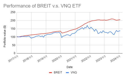
Figure 1. Private real estate (BREIT) v.s. public real estate (VNQ ETF), January 2017 - March 2024.

Some statistics²⁸ for these two funds:

Instrument	Annualized Mean	Annualized Standard Deviation	Annualized Sharpe Ratio	First-order autocorrelation
BREIT	10.10%	4.58%	2.20	0.42
VNQ ETF	6.26%	18.68%	0.34	-0.13

From Figure 1 and the associated statistics (e.g., one-fourth of the volatility of its public counterpart, strong first-order autocorrelation), BREIT is a textbook case of volatility laundering that we can combat thanks to Geltner’s procedure²⁹!

Figure 2 depicts the resulting unsmoothed BREIT together with the original BREIT and the VNQ ETF.

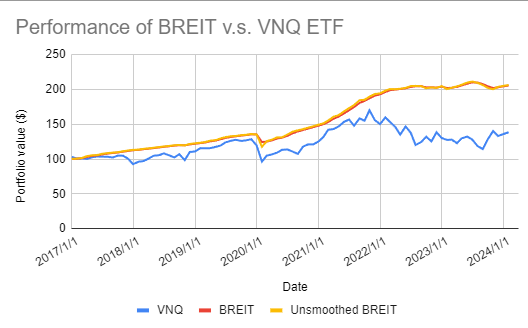
Figure 2. Smoothed and unsmoothed private real estate (BREIT) v.s. public real estate (VNQ ETF), January 2017 - March 2024.

Some additional statistics for the unsmoothed BREIT:

Instrument	Annualized Mean	Annualized Standard Deviation	Annualized Sharpe Ratio	First-order autocorrelation
Unsmoothed BREIT	10.28%	6.85%	1.50	-0.04

While Figure 2 is hardly distinguishable from Figure 1, the associated statistics are clear and consistent with the litterature:

Unsmoothing the returns of BREIT increases its volatility by nearly 50%
Unsmoothing the returns of BREIT also decreases its annualized Sharpe Ratio by approximately 30%

This small exercice empirically validates that unsmoothing private asset returns makes them look and feel more like a public market proxy³⁰.

To be noted that the unsmoothed BREIT still seems a little bit too smooth when compared to the VNQ ETF.

Analysing hedge funds returns

Brooks and Kat¹⁸, as well as many other authors¹¹⁹²¹³¹, observes that hedge funds exhibit significant levels of first - and sometimes second or higher - order autocorrelation, which has important consequences for investors¹⁸.

In particular, and thanks to the unsmoothing procedures previously described:

Gallais-Hamonno and Nguyen-Thi-Thanh²¹ notes that

[…] the hedge fund performance measured by traditional ratios considerably decreases after unsmoothing, decrease which is on average 20%, even 25% according to the method and to the performance ratio used.

[…] 20% of [hedge funds] have a change in rankings. Moreover, there are several cases of strong “down-grading” and of strong “over-grading” […]
Okunev and White¹⁹ shows that

After removing the autocorrelations from returns, we find increases in risk of between 60 and 100 percent for many of the individual indices.

So, when analysing hedge funds returns, a pre-requisite is to always use an unsmoothing procedure!

Mitigating covariance misspecification in asset allocation

In the context of a multi-asset portfolio, Peterson and Grier² shows through a Monte Carlo mean-variance experiment that the naive covariance estimates [relying on smoothed asset returns] generate significant weight bias, undesirable allocative tilts, and higher portfolio risk².

Similar in spirit to that paper, I propose to illustrate the impact of smoothed returns on mean-variance analysis.

For this:

I consider a U.S.-centric universe of assets made of five Preqin private investment indexes and their public markets equivalents:
- Private Equity and S&P 500 index
- Venture Capital and Russell 2000 index
- Private Debt and an High Yield Bonds index³²
- Private Real Estate and MSCI U.S. Real Estate index
- Private Infrastructure and S&P Infrastructure index
  
  Figure 3 displays the (quarterly) evolution of all these indexes over the period 31 December 2007 - 31 December 2023.
  
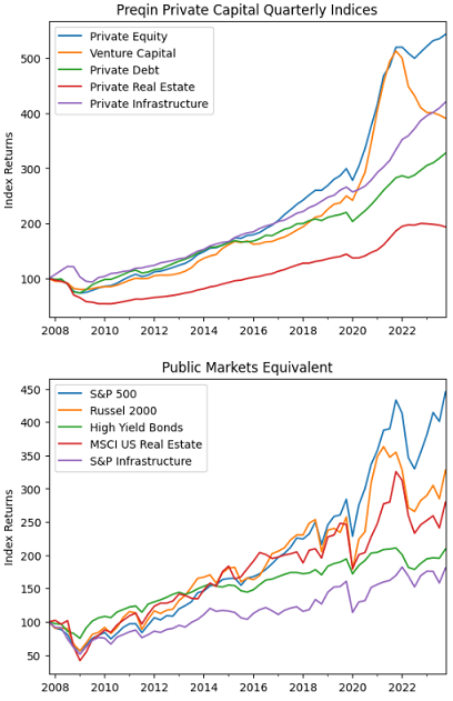
  Figure 3. Private investment indexes v.s. public markets equivalents, 31 December 2007 - 31 December 2023.
Within that universe, I then compute two mean-variance efficient frontiers over the period 31 December 2007 - 31 December 2023, using in-sample annualized mean-variance inputs³³:
- A “raw” efficient frontier, using reported returns for all indexes
- An “unsmoothed” efficient frontier, using unsmoothed³⁴ reported returns for the private investment indexes and reported returns for their public markets equivalents
  
  Figure 4 represents these two efficient frontiers in the mean-variance plane, together with the different indexes of the considered universe.
  
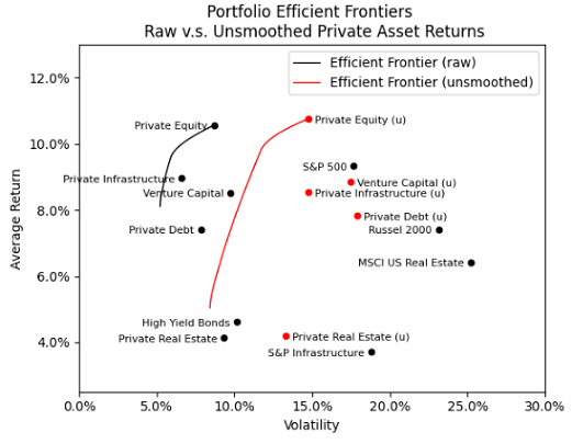
  Figure 4. Efficient frontiers for raw v.s. unsmoothed private investment indexes, 31 December 2007 - 31 December 2023.
  
  From Figure 4, and in accordance with Peterson and Grier²:
  - The standard deviations of the private investment indexes increase significantly when their reported returns are unsmoothed.
  - The difference in the locations of the two frontiers is largely³⁵ a result of the underestimated standard deviations of the smoothed [private investment indexes]².
  This confirms that the naive covariance matrix underestimates risk and overestimates returns relative to the more efficient revised covariance matrix² and that unsmoothing is necessary to remove potential biases and improve efficiency by maximizing the information content of [the mean-variance input] estimates².
  
  One important remark, though, is that the unsmoothing procedure used only partially resolved the issues related to smoothed asset returns.
  
  Indeed, the transition maps³⁶ of the two efficient frontiers (Figure 5) shows that unsmoothed mean-variance efficient portfolios are still heavily concentrated in private assets…
  
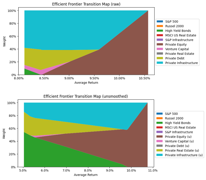
  Figure 5. Transition maps of efficient frontiers for raw v.s. unsmoothed private investment indexes, 31 December 2007 - 31 December 2023.
  
  So, to paraphrase Trym Riksen, private assets break the Markovitz’s model, and do so even when their “specificities” are accounted for!
  
  More on this right now.

Conclusion

A proper conclusion is certainly that in general, [private asset returns] series must be unsmoothed before analysis² to avoid introducing any unwanted bias.

Nevertheless, the two unsmoothing procedures described in this blog post are not entirely satisfying because the resulting unsmoothed returns are yet too smooth…

Next in this series on combating volatility laundering, I will describe another unsmoothing procedure, this time able to take into account³⁷ the economic relationship between a private asset and its public market equivalent, which might improve its practical performances.

In order to smoothly stay up-to-date with I am doing, feel free to connect with me on LinkedIn or to follow me on Twitter.

–

See Mila Getmansky, Andrew W. Lo, Igor Makarov, An econometric model of serial correlation and illiquidity in hedge fund returns, Journal of Financial Economics, Volume 74, Issue 3, 2004, Pages 529-609. ↩ ↩² ↩³ ↩⁴ ↩⁵ ↩⁶
See Steven P. Peterson and John T. Grier, Covariance Misspecification in Asset Allocation, Financial Analysts Journal, Vol. 62, No. 4 (Jul. - Aug., 2006), pp. 76-85. ↩ ↩² ↩³ ↩⁴ ↩⁵ ↩⁶ ↩⁷ ↩⁸ ↩⁹ ↩¹⁰
See Venables, W. N. and Ripley, B. D. (2002) Modern Applied Statistics with S. Fourth Edition. Springer-Verlag. ↩ ↩²
See On the Autocorrelation of the Stock Market, Ian Martin, Journal of Financial Econometrics, Volume 19, Issue 1, Winter 2021, Pages 39–52. ↩
See Samuelson P. A. 1965. Proof That Properly Anticipated Prices Fluctuate Randomly. Industrial Management Review 6: 41–49. ↩
Campbell, R., 2008. Art as a financial investment. Journal of Alternative Investments 10, 64–81. ↩
See Dimson, Elroy, and Christophe Spaenjers. 2011. Ex post: The investment performance of collectible stamps. Journal of Financial Economics 100:443–458. ↩
See Ang, A., Chen, B., Goetzmann, W. N., Phalippou, L., 2018. Estimating private equity returns from limited partner cash flows. The Journal of Finance 73, 1751–1783. ↩
See Alexander D. Beath, PhD and Chris Flynn, CFA, ASSET ALLOCATION, COST OF INVESTING AND PERFORMANCE OF EUROPEAN DB PENSION FUNDS: THE IMPACT OF REAL ESTATE, CEM Benchmarking Inc.. ↩ ↩²
See Geltner, David, 1991, Smoothing in Appraisal-Based Returns, Journal of Real Estate Finance and Economics, Vol.4, p.327-345, Geltner, David, 1993, Estimating Market Values from Appraised Values without Assuming an Efficient Market, Journal of Real Estate Research, Vol.8, p.325-345 and Fisher, J. D., Geltner, D. M., & Webb, R. B. (1994). Value indices of commercial real estate: A comparison of index construction methods. The Journal of Realv Estate Finance and Economics, 9 (2), 137–164. ↩ ↩² ↩³ ↩⁴ ↩⁵ ↩⁶ ↩⁷
See Verdickt, Gertjan, Volatility Laundering: On the Feasibility of Wine Investment Funds (March 28, 2024). ↩ ↩²
In the context of hedge funds. ↩ ↩²
See Spencer J Couts, Andrei S Gonçalves, Andrea Rossi, Unsmoothing Returns of Illiquid Funds, The Review of Financial Studies, 2024. ↩ ↩²
See Antti Ilmanen, Investing in Interesting Times, The Journal of Portfolio Management, Multi-Asset Special Issue 2023, 49 (4) 21 - 35. ↩
See Cliff Asness, Volatility Laundering, Perspective. ↩
In the context of private equity, c.f. the podcast Private Equity and the Game of ”Volatility Laundering” from This Week in Intelligent Investing. ↩
Or volatility laundered. ↩
See Brooks, C. and H. Kat, The statistical properties of Hedge Fund index returns and their implications for investors, The Journal of Alternative Investments, Fall 2002, 5 (2) 26-44. ↩ ↩² ↩³
See Geoff Loudon, John Okunev, Derek White, Hedge Fund Risk Factors and the Value at Risk of Fixed Income Trading Strategies, The Journal of Fixed Income, Fall 2006, 16 (2) 46-61 and Okunev, John and White, Derek, Hedge Fund Risk Factors and Value at Risk of Credit Trading Strategies (October 2003). ↩ ↩² ↩³ ↩⁴ ↩⁵ ↩⁶ ↩⁷ ↩⁸ ↩⁹ ↩¹⁰ ↩¹¹
See Shilling, James D. Measurement Error in FRC/NCREIF Returns on Real Estate. Southern Economic Journal, vol. 60, no. 1, 1993, pp. 210–19. ↩
See Georges Gallais-Hamonno, Huyen Nguyen-Thi-Thanh. The necessity to correct hedge fund returns: empirical evidence and correction method. 2007. ↩ ↩² ↩³
For example, use the time series [-0.94, -0.96, -0.98, -0.95]. ↩
Called i.i.d.-based in de Prado²⁵. ↩
See Lo, A. W., 2002. The statistics of sharpe ratios. Financial Analysts Journal 58, No. 4, 36–52. ↩
See Bailey, David H. and Lopez de Prado, Marcos, Stop-Outs Under Serial Correlation and ‘The Triple Penance Rule’. ↩ ↩²
See The Case Against Private Markets. ↩ ↩²
(Adjusted) prices have have been retrieved using Tiingo. ↩
Due to the first-order autocorrelation in BREIT returns, the naive annualization of the volatility and of the Sharpe Ratio that I have done is incorrect, c.f. Lo²⁴; this is done on purpose, though. ↩
Okunev and White’s procedure gives nearly identical results. ↩
See Bingxu Chen & Christopher Carrano, Two Easy Steps to Take Your Private Asset Returns Public, Vnn by Two Sigma. ↩
See Clifford S Asness, Robert J Krail, John M Liew, Do Hedge Funds Hedge?, The Journal of Portfolio Management, Fall 2001, 28 (1) 6-19. ↩
The associated index is the Markit iBoxx USD Liquid High Yield Index; comparison of Private Debt to both Investment Grade and High Yield bonds is discussed in Boni and Manigart³⁸. ↩
In-sample asset mean returns and in-sample asset returns covariance matrix, using asset returns over the period 31 March 2008 - 31 December 2023. ↩
Reported returns for the private investment indexes were unsmoothed using the Okunev and White’s procedure of order 1; results are similar with Geltner’s procedure, but since I already used Geltner’s procedure in the context of real-estate, I decided to play with its extension. ↩
To be noted that the in-sample asset mean returns are numerically different between smoothed and unsmoothed returns, but this does not explain the differences between the two frontiers. ↩
The transition map of the efficient frontier is a stacked area plot of the composition, in terms of asset weights, of the efficient portfolios belonging to the efficient frontier. ↩
That being said, a variant of Geltner’s method allow to use a public market equivalent of a private asset to “inject” volatility in the unsmoothed returns, c.f. Geltner¹⁰. ↩
See Boni, Pascal and Manigart, Sophie, Private Debt Fund Returns, Persistence, and Market Conditions. ↩