Completing a Correlation Matrix: Another Problem from Finance

The previous post of this series on mathematical problems related to correlation matrices introduced the nearest correlation matrix problem¹, which consists in determining the closest² valid correlation matrix to an approximate correlation matrix

In this blog post, I will now describe the correlation matrix completion problem, which consist in filling in the missing coefficients of a partially specified correlation matrix in order to produce a valid correlation matrix.

As noted in Dreyer et al.³, such matrices often arise in financial applications when the number of stochastic variables becomes large or when several smaller models are combined in a larger model³.

After a couple of reminders on correlation matrices, I will detail the mathematical formulation of the correlation matrix completion problem, discuss its exact and approximate solutions and I will finally illustrate how this problem naturally appears when working with capital market assumptions from financial institutions.

Mathematical preliminaries

Let $n$ be a number of assets.

Correlation matrices

Let $C \in \mathcal{M} \left( \mathbb{R}^{n \times n} \right)$ be a square matrix.

$C$ is a correlation matrix if and only if

• $C$ is symmetric: $C {}^t = C$
• $C$ is unit diagonal: $C_{i,i} = 1$, $i=1..n$
• $C$ is positive semi-definite, that is, $x {}^t C x \geqslant 0, \forall x \in \mathbb{R}^n $

The sets of correlation matrices

Let be the following convex sets:

• $\mathcal{S}^n_{+} = \{ X \in \mathcal{M} \left( \mathbb{R}^{n \times n} \right)$ such that $X {}^t = X$ and $X$ is positive semi-definite $\}$
• $\mathcal{S}^n_{++} = \{ X \in \mathcal{M} \left( \mathbb{R}^{n \times n} \right)$ such that $X {}^t = X$ and $X$ is positive definite $\}$
• $\mathcal{E}^n = \{ X \in \mathcal{M} \left( \mathbb{R}^{n \times n} \right)$ such that $X {}^t = X$ and $x_{ii} = 1, i = 1,…,n \}$

Then:

• The set of correlation matrices is the convex compact set $\mathcal{S}^n_{+} \cap \mathcal{E}^n$.
• The set of invertible correlation matrices is the open bounded convex set $\mathcal{S}^n_{++} \cap \mathcal{E}^n$.

As a geometrical side note, the set of vectorized correlation matrices defines a subset of the unit hypercube in $\mathbb{R}^n$ called the elliptope, c.f. for example the website Convex Optimization.

Partial correlation matrices completion

A partial correlation matrix $C \in \mathcal{M} \left( \mathbb{R}^{n \times n} \right)$ is a symmetric unit diagonal matrix⁴ whose coefficients $c_{ij} = c_{ji}$ are not all specified.

A partial correlation matrix is said to be partial positive (semi-)definite when its specified principal minors are positive (semi-)definite.

A positive semi-definite completion - or simply a completion - of a partial correlation matrix $C \in \mathcal{M} \left( \mathbb{R}^{n \times n} \right)$ is a correlation matrix $C^* \in \mathcal{M} \left( \mathbb{R}^{n \times n} \right)$ such that $c_{ij}^{*} = c_{ij}$ whenever the coefficient $c_{ij}$ is specified in $C$.

A positive definite completion of a partial correlation matrix $C \in \mathcal{M} \left( \mathbb{R}^{n \times n} \right)$ is a positive definite correlation matrix $C^* \in \mathcal{M} \left( \mathbb{R}^{n \times n} \right)$ such that $c_{ij}^{*} = c_{ij}$ whenever the coefficient $c_{ij}$ is specified in $C$.

Undirected graph associated to a correlation matrix

Let $C \in \mathcal{M} \left( \mathbb{R}^{n \times n} \right)$ be a partial correlation matrix.

It is possible⁵ to associate an undirected graph $G = \left( V, E \right)$ to $C$, defined as follows:

• $V = \{ 1, 2, …, n \}$ is the set of vertices
• $E$ is the set of edges, with $(i,j) \in E$ whenever the coefficient $c_{ij}$ is specified, with $i \ne j$.

The graph $G$ is then said to be chordal if every cycle of length greater than or equal to 4 has a chord, which is an edge that is not part of the cycle but connects two vertices of the cycle⁶.

As a reminder, a cycle in G is a sequence of $k \geq 3$ pairwise distinct vertices $\left( v_1, …, v_s \right)$ such that $\left( v_1, v_2 \right)$, $\left( v_2, v_3 \right)$, …, $\left( v_{k-1} v_k \right)$, $\left( v_k v_1 \right)$ $\in E$, with $k$ called the length of the cycle.

The correlation matrix completion problem

Problem formulation

Let be:

• $C \in \mathcal{M} \left( \mathbb{R}^{n \times n} \right)$ a partial correlation matrix.
• $\mathcal{N}$ the index set of the specified off-diagonal elements of $C$.
• $\mathcal{U}^n = \{ X \in \mathcal{M} \left( \mathbb{R}^{n \times n} \right)$ such that $x_{ij}=c_{ij}$ for $(i,j) \in \mathcal{N} \}$

Then:

• The correlation matrix completion problem is the problem of finding a correlation matrix $C^* \in \mathcal{M} \left( \mathbb{R}^{n \times n} \right)$ that completes the matrix $C$, that is, finding $C^* \in \mathcal{S}^n_{+} \cap \mathcal{U}^n$.
• The positive definite correlation matrix completion problem is the problem of finding a positive definite correlation matrix $C^* \in \mathcal{M} \left( \mathbb{R}^{n \times n} \right)$ that completes the matrix $C$, that is, finding $C^* \in \mathcal{S}^n_{++} \cap \mathcal{U}^n$.

Existence of solutions

Contrary to the nearest correlation matrix problem, the correlation matrix completion problem does not always admit a solution.

Indeed, an already necessary condition for a completion to exist is for the partial correlation matrix to be partial positive semi-definite⁵.

So, for example, the following partial correlation matrix does not admit any completion:

\[C_1 = \begin{pmatrix} 1 & -1 & -1 & -1 \\ -1 & 1 & -1 & -1 \\ -1 & -1 & 1 & . \\ -1 & -1 & . & 1 \end{pmatrix}\]

Beyond this necessary condition, Fiedler⁷, Grone et al.⁵ and Smith⁸ all establish the following result⁹:

A partial positive semi-definite correlation matrix is completable regardless of the values of the specified correlations if and only if the undirected graph associated to these specified correlations is chordal.

To be noted that when that graph is not chordal, nothing can be said in general because the existence of a completion then depends on the exact values of the specified correlations.

As an illustration:

• Let $C_2 \in \mathcal{M} \left( \mathbb{R}^{4 \times 4} \right)$ be the following partial positive definite correlation matrix:

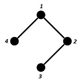
  \[C_2 = \begin{pmatrix} 1 & 1 & . & 1 \\ 1 & 1 & 1 & . \\ . & 1 & 1 & . \\ 1 & . & . & 1 \end{pmatrix}\]

  The undirected graph associated to that partial correlation matrix is the graph with the set of vertives $V = \{ 1, 2, 3, 4 \}$ and the set of edges $G = \{ (1,2), (1,4), (2,3) \}$, depicted in Figure 1.

  

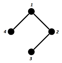
  Figure 1. Undirected graph associated to the partial correlation matrix C2.

  From Figure 1, that graph is chordal, because there are no cycles of length >= 4.

  Consequently, the partial correlation matrix $C_2$ admit a positive definite completion and the existence of that completion does actually even not depend on the values of the specified correlations (here, all 1s).

• Let now $C_3 \in \mathcal{M} \left( \mathbb{R}^{4 \times 4} \right)$ be the following partial positive semi-definite correlation matrix:

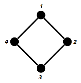
  \[C_3 = \begin{pmatrix} 1 & 1 & . & 0 \\ 1 & 1 & 1 & . \\ . & 1 & 1 & 1 \\ 0 & . & 1 & 1 \end{pmatrix}\]

  The undirected graph associated to that partial correlation matrix is the graph with the set of vertives $V = \{ 1, 2, 3, 4 \}$ and the set of edges $G = \{ (1,2), (1,4), (2,3), (3,4) \}$, depicted in Figure 2.

  

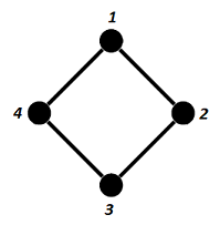
  Figure 2. Undirected graph associated to the partial correlation matrix C3.

  From Figure 2, that graph is not chordal, because there is only one cycle of length 4 and that cycle does not have any chord.

  Consequently, the partial correlation matrix $C_3$ might or might not admit a completion, nothing can be said at this stage.

For the interested reader, a couple of other theoretical results can be found in Fiedler⁷, which also notes that the general [completion] problem […] seems to be difficult⁷.

Unicity of solutions

Again contrary to the nearest correlation matrix problem, the correlation matrix completion problem does not generally admit a unique solution when one exists.

Indeed, Grone et al.⁵ establishes that the set of all positive semi-definite completions of a partial correlation matrix is in general a convex compact set and not a singleton.

This result can be illustrated with one and two missing correlations:

• One missing correlation

  The partial correlation matrix $C_4 = \begin{pmatrix} 1 & . \\ . & 1 \end{pmatrix} $ has one missing correlation.

  By introducing the variable $x$ representing that missing correlation, a completion is a valid completion if and only if it has a positive or null determinant, that is, $\det(x) = 1 - x^2 \geq 0$.

  That condition being equivalent to the condition $x \in [-1,1]$, all correlation matrices of the form $ C^*_4(x) = \begin{pmatrix} 1 & x \\ x & 1 \end{pmatrix} $ with $x \in [-1,1]$ are completions of $C_4$.

• Two missing correlations

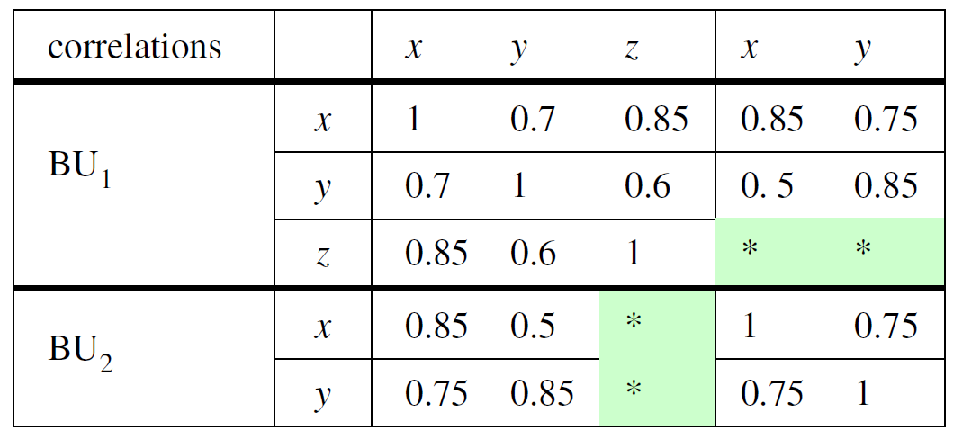
  The partial correlation matrix $C_5 \in \mathcal{M} \left( \mathbb{R}^{5 \times 5} \right)$ represented in Figure 3 has two missing correlations.

  

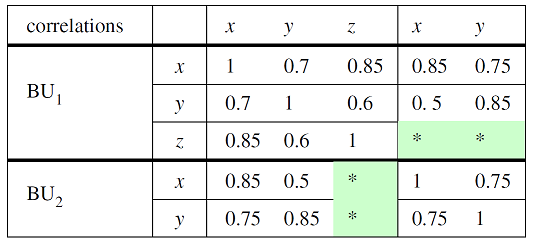
  Figure 3. Partial correlation matrix with 2 missing correlations. Source: Georgescu et al.

  Because all the specified sub-matrices of $C_5$ are positive semi-definite, a completion is again a valid completion if and only if it has a positive or null determinant.

  By introducing the variables $x$ and $y$ representing the two missing correlations, the determinant of $C_5$ can be factored as $ \det(x,y) $ $ \approx$ $ −0.18 \left( 0.67x^2 +0.75y^2 −xy −0.32x−0.24y+0.17 \right)$.

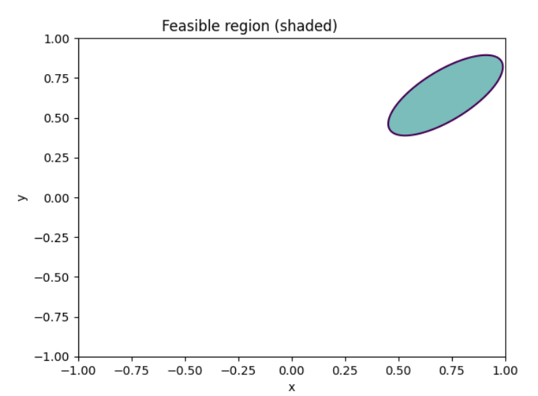
  Non-negativity of that determinant is then equivalent to the condition

  \[0.67x^2 +0.75y^2 −xy −0.32x−0.24y+0.17 \leq 0\]

  , which defines the 2-dimensional ellipse (and its interior) depicted in Figure 4.

  

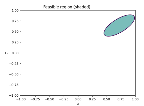
  Figure 4. Feasible region for Georgescu et al.'s partial correlation matrix completions.

  All correlation matrices $C_5^{*}(x,y) \in \mathcal{M} \left( \mathbb{R}^{5 \times 5} \right)$ with the same correlations as $C_4$, a correlation $c^{*}_{34}$ $=$ $x$ and a correlation $c^{*}_{35}$ $=$ $y$ - with $x,y$ satisfying the above relationship - are thus completions of $C_5$.

The existence of infinitely many completions¹⁰ naturally leads to trying to find a best-estimate completion in some sense⁶, which does exist and is called the maximum determinant completion⁶.

The maximum determinant correlation matrix completion problem

Fiedler⁷ originally demonstrated that if a positive definite partial correlation matrix admits a completion, then, there is a unique matrix in the (nonempty) class of all positive definite completions […] that has maximum determinant⁸.

More recently, by introducing a generalized determinant that gives the determinant of the nonsingular part of [a] matrix¹¹, Dreyer¹¹ established a similar result for positive semi-definite partial correlation matrices.

That completion, called the maximum determinant completion - or the Max-Det completion - has several intesting theoretical properties, which makes it an ideal candidate for guaranteeing the unicity of the completion of a correlation matrix.

Problem formulation

Let be:

• $C \in \mathcal{M} \left( \mathbb{R}^{n \times n} \right)$ a partial correlation matrix.
• $\mathcal{N}$ the index set of the specified off-diagonal elements of $C$.
• $\mathcal{U}^n = \{ X \in \mathcal{M} \left( \mathbb{R}^{n \times n} \right)$ such that $x_{ij}=c_{ij}$ for $(i,j) \in \mathcal{N} \}$

The maximum determinant correlation matrix completion problem can be cast as a generalization of a semidefinite programming problem:

\[C^* = \operatorname{argmax} \log ( \det (X) ) \text{ s.t. } X \in \mathcal{S}^n_{+} \cap \mathcal{E}^n \cap \mathcal{U}^n\]

Assuming that a solution exist, c.f. the previous section, Grone et al.⁵ and Olvera Astivia¹² show using standard results from mathematical optimization theory that it is necessarily unique.

Mathematical properties of the solution

Georgescu et al.⁶ summarizes the main properties of the maximum determinant correlation matrix completion:

• For the multivariate normal model, it maximizes the entropy of the distribution described by the matrix

  van der Schans and Boer¹³ comments this property as follows:

  Since the already specified [correlations] imply a dependence between variables between which no dependence is specified and dependence reduces the amount of uncertainty in a system, the intuitive interpretation of entropy maximization is not introducing more dependence than is already implied by the already specified [correlations].

• Again for the multivariate normal model, it maximizes the likelihood of the correlation matrix

• It corresponds to the analytic centre of the feasible region described by the positive semi-definiteness constraints⁶

  In other words, for a given partial correlation matrix, its maximum determinant completion lies as “deep” as possible¹⁴ inside the set of all its positive definite completions.

Computation of the solution

The original algorithmic approach to solving determinant maximization problems with matrix constraints has been to use interior point methods¹⁵.

More recently, dual projected gradient methods have been developed that are better able to scale with the dimensionality of the problem¹⁶.

Nevertheless, the drawbacks of these algorithms, from an application point of view, are that they are difficult to implement […], do not always converge if inconsistent starting [correlations] are specified and, finally, global optimization is too slow and memory consuming for large matrices¹³.

More on “inconsistent starting correlations” later.

For these reasons, it is tempting to [simply] set the missing [correlations] to zero³, but this approach has several shortcomings³, among which the fact that forcing unspecified correlations to zero¹⁷ might not be ideal for financial applications where most assets are correlated to each other.

To illustrate this point, Figure 5 represents a partial correlation matrix with a block of missing correlations.

Figure 5. Partial correlation matrix with a block of missing correlations. Source: Georgescu et al.

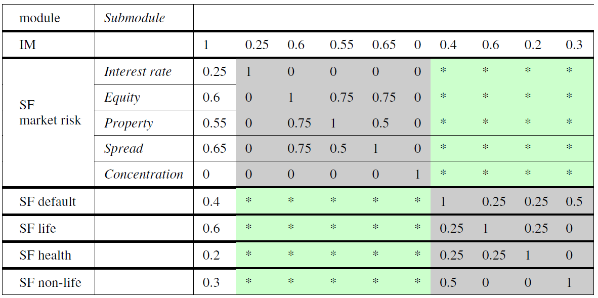
The maximum determinant completion of the block of missing correlations is⁶

\[E_1 = \begin{pmatrix} 0.1000 & 0.1500 & 0.0500 & 0.0750 \\ 0.2400 & 0.3600 & 0.1200 & 0.1800 \\ 0.2200 & 0.3300 & 0.1100 & 0.1650 \\ 0.2600 & 0.3900 & 0.1300 & 0.1950 \\ 0 & 0 & 0 & 0 \end{pmatrix}\]

, while the completion of the same block of missing correlations obtained after setting them to zero and computing the nearest correlation matrix to the resulting full approximate correlation matrix is⁶

\[E_2 = \begin{pmatrix} 0.0022 & 0.0084 & 0.0004 & 0.0035 \\ 0.0003 & 0.0011 & 0.0001 & 0.0005 \\ 0.0025 & 0.0098 & 0.0005 & 0.0040 \\ 0.0042 & 0.0164 & 0.0008 & 0.0067 \\ 0 & 0 & 0 & 0 \end{pmatrix}\]

Comparing the two sub-matrices $E_1$ and $E_2$, it is clear that the completed correlations of $E_2$ are much closer to zero than those of $E_1$, thus imposing an additional soft constraint of “closeness to zero” to the correlation matrix completion problem.

Reverting to simple heuristics for the correlation matrix completion problem might thus be potentially dangerous, depending on the context.

Hopefully, van der Schans and Boer¹³ proposes an heuristic which does not suffer from these shortcomings and that:

• Is fast, which makes it suitable for applications in which the computation time is important¹³
• Tries to not introduce more dependence between variables than is implied by the initially specified [correlations]¹³, contrary to the “setting missing correlations to zero” heuristic
• Additionally corrects for inconsistencies in the already specified [correlations]¹³, but again, more on this later
• Empirically produces completions with an average correlation difference with the maxdet completion [that is] reasonable¹³

A drawback of this heuristic, though, is that it depends on the ordering of the rows and columns of the [correlation] matrix, i.e. the heuristic will yield a different result if first rows and columns of [the matrix] are interchanged before starting the procedure¹³, which might or might not be acceptable in practice.

As a side note, explicit solutions of the maximum determinant correlation matrix completion problem are known in specific cases, for example for correlation matrices that follow an L-shaped, block diagonal pattern which is a common structure in insurance problems¹², c.f. Georgescu et al.⁶

The infeasible maximum determinant correlation matrix completion problem

In the previous section, a solution to the maximum determinant correlation matrix completion problem was assumed to exist.

There are at least two practical problems with this assumption:

• A partial correlation matrix might theoretically admit a completion, but numerical round-off errors might prevent an algorithm from finding it

  An example of such an ill-behaved matrix can be found in Glunt et al.¹⁸, but it is a partial covariance matrix and not a partial correlation matrix…

  Building a similar example using a partial correlation matrix is certainly doable, but I failed to do so quickly, so, no example here.

• More typically, the initially specified [correlations] can be inconsistent in the sense that no valid completion exists¹³

  Here, the partial correlation matrix $C_1$ perfectly illustrates this point, even though it is a rather extreme example.

In both cases, simply failing to compute a solution might be unacceptable (e.g. for downstream pipelines), so that something must be done.

Unfortunately, the currently existing literature does not focus on algorithms that both complete partially specified matrices and also correct for inconsistencies¹³.

In other words, there is no well-established formulation of what could be called the infeasible maximum determinant correlation matrix completion problem.

At minimum, what can be said is that any solution to this new problem must involve a trade-off between

• The closeness to the initial partial correlation matrix, for example in terms of the Frobenius distance
• The value of the determinant

Incidentally, this is exactly how the heuristic algorithm of van der Schans and Boer¹³ is working: the specified [correlations] are adjusted as little as possible¹³ and the introduced extra (conditional) dependence between variables is as little as possible¹³.

When applied to the partial correlation matrix $C_1$, van der Schans and Boer’s algorithm¹³ gives

\[C^*_1 = \begin{pmatrix} 1 & -0.99 & -0.07 & -0.07 \\ -0.99 & 1 & -0.07 & -0.07 \\ -0.07 & -0.07 & 1 & 0.98 \\ -0.07 & -0.07 & 0.98 & 1 \end{pmatrix}\]

As expected, the completed correlation matrix $C^*_1$ is very far from the partial correlation matrix $C_1$, with only one correlation close to its initial value of -1 (-0.99).

Again, this is an extreme infeasible example, but it empirically demonstrates that adjusting the initially specified correlations, even as little as possible¹³, can lead to a completed correlation matrix that does not ressemble at all the initial partial correlation matrix.

Implementation in Portfolio Optimizer

Portfolio Optimizer implements two methods to complete a partial correlation matrix through the endpoint /assets/correlation/matrix/completed:

• One proprietary method that guarantees to find the maximum determinant completion if it exists or that guarantees to minimally adjust - in terms of Frobenius distance - the partially specified correlation matrix so that a maximum determinant completion exists
• The heuristic method of van der Schans and Boer¹³, with additional tweaks to improve its numerical robustness

For comparison with van der Schans and Boer’s algorithm¹³, the proprietary method of Portfolio Optimizer applied to the partial correlation matrix $C_1$ gives:

\[C^{**}_1 = \begin{pmatrix} 1 & -0.30 & -0.59 & -0.59 \\ -0.30 & 1 & -0.59 & -0.59 \\ -0.59 & -0.59 & 1 & 1 \\ -0.59 & -0.59 & 1 & 1 \end{pmatrix}\]

Comparing the two completed matrices $C_1^{*}$ and $C_1^{**}$, it appears that the matrix $C_1^{**}$ is much¹⁹ closer to the partial correlation matrix $C_1$ than the matrix $C_1^{*}$, which is consistent with the expected behaviour of Portfolio Optimizer.

Example of usage - Completing partial correlation matrices from financial institutions

Major financial institutions regularly provide forecasts of future risk/return characteristics for broad asset classes over the next 5 to 20 years, called (Long Term) Capital Market Assumptions (LTCMA).

In addition to the future expected volatility, the risk forecasts sometimes also include future expected correlation matrices, which is for example the case with J.P. Morgan.

Unfortunately, these correlation matrices are typically partially specified.

In addition, even if they were fully specified, combining capital market assumptions from several financial institutions would render them partial due to all institutions not covering the same asset classes…

So, as an example of usage, I propose to compute the maximum determinant completion of the partial correlation matrix provided by Blackrock as part of their November 2025 5-year capital market assumptions and represented in Figure 6.

Figure 6. Five-year expected future partial correlations between major asset classes, NZD currency, 13th November 2025. Source: Blackrock.

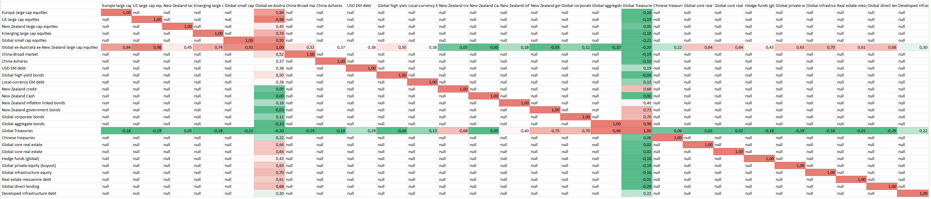
The resulting maximum determinant completed correlation matrix is displayed in Figure 7.

Figure 7. Five-year expected future Max-Det completed correlations between major asset classes, NZD currency, 13th November 2025.

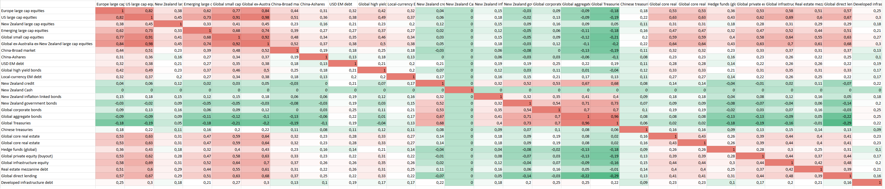
I would like to mention that such an example of usage was inspired by a LinkedIn post from Peter Urbani, who proposes to complete Blackrock’s partial correlation matrix into the correlation matrix displayed in Figure 8 thanks to a 2-factor model built from the fully specified global equities/global bonds correlations.

Figure 8. Five-year expected future 2-factor model completed correlations between major asset classes, NZD currency, 13th November 2025. Source: Peter Urbani.

Comparing the “Max-Det” completed correlation matrix with Peter Urbani’s “2-factor model” completed correlation matrix , both matrices are perfectly identical²⁰.

As a closing (fun) remark, Olvera Astivia¹² highlights that having half of the entries in a correlation matrix missing [can be] considered a rather extreme condition¹².

What could then be said about the initial Blackrock’s partial correlation matrix that has around 82% of missing entries?!

Conclusion

With this first blog post of 2026, my hope is that you have added to your quantitative toolbox a useful methodology to obtain, in a mathematically principled way, values implied in correlational structure of the data, even if said data has not (or cannot) be obtained¹².

In any cases, for more mathematics of correlation matrices, feel free to connect with me on LinkedIn or to follow me on Twitter.

–

1. Nicholas J. Higham, Computing the Nearest Correlation Matrix—A Problem from Finance, IMA J. Numer. Anal. 22, 329–343, 2002.. ↩

2. In terms of the Frobenius distance. ↩

3. Olaf Dreyer, Horst Kohler, Thomas Streuer, Completing correlation matrices, arXiv. ↩ ↩² ↩³ ↩⁴

4. That is, belonging to the set $\mathcal{E}^n$. ↩

5. R. Grone, C.R. Johnson, E. Sa, H. Wolkowicz, Positive definite completions of partial Hermitian matrices, Linear Algebra Appl. 58 (1984) 109–124. ↩ ↩² ↩³ ↩⁴ ↩⁵

6. Georgescu DI, Higham NJ, Peters GW. 2018 Explicit solutions to correlation matrix completion problems, with an application to risk management and insurance. ↩ ↩² ↩³ ↩⁴ ↩⁵ ↩⁶ ↩⁷ ↩⁸

7. Fiedler, M. Matrix Inequalities. Numer. Math. 9, 109–119 (1966). ↩ ↩² ↩³ ↩⁴

8. Ronald L. Smith, The positive definite completion problem revisited, Linear Algebra and its Applications, Volume 429, Issue 7, 2008,Pages 1442-1452. ↩ ↩²

9. One interesting feature of that result is that the existence of a correlation matrix completion - which seems quite algebric in nature - is actually equivalent to a “visual” condition. ↩

10. When one exists. ↩

11. Olaf Dreyer, Matrix completion and semidefinite matrices, arXiv. ↩ ↩²

12. Oscar L. Olvera Astivia (2021) A Note on the General Solution to Completing Partially Specified Correlation Matrices, Measurement: Interdisciplinary Research and Perspectives, 19:2, 115-123. ↩ ↩² ↩³ ↩⁴ ↩⁵

13. See van der Schans, Martin and Boer, Alex, A Heuristic for Completing Covariance And Correlation Matrices (March 14, 2013). Technical Working Paper 2014-01 November 2014. ↩ ↩² ↩³ ↩⁴ ↩⁵ ↩⁶ ↩⁷ ↩⁸ ↩⁹ ↩¹⁰ ↩¹¹ ↩¹² ↩¹³ ↩¹⁴ ↩¹⁵ ↩¹⁶ ↩¹⁷

14. The maximum determinant correlation matrix completion maximizes the product of distances to the defining hyperplanes⁶. ↩

15. See Vandenberghe, Lieven and Boyd, Stephen and Wu, Shao-Po, Determinant Maximization with Linear Matrix Inequality Constraints, SIAM Journal on Matrix Analysis and Applications, Volume 19, Number 2, Pages 499-533. ↩

16. See Nakagaki, T., Fukuda, M., Kim, S. et al. A dual spectral projected gradient method for log-determinant semidefinite problems. Comput Optim Appl 76, 33–68 (2020). ↩

17. Or close to zero in case the nearest correlation matrix to the resulting approximate correlation matrix is computed. ↩

18. W. Glunt, T.L. Hayden, Charles R. Johnson, P. Tarazaga, Positive definite completions and determinant maximization, Linear Algebra and its Applications, Volume 288, 1999, Pages 1-10. ↩

19. The Frobenius distance between $C_1$ and $C^*_1$ is $\approx 2.630$, while the Frobenius distance between $C_1$ and $C^{**}_1$ is $\approx 1.575$. ↩

20. Incidentally, this allows to conclude - due to the entropy maximization property of the maximum determinant correlation matrix completion under a multivariate normal model - that the 2-factor model used by Peter Urbani is a vanilla multivariate normal model. ↩