Cluster Risk Parity: Equalizing Risk Contributions Between and Within Asset Classes
The equal risk contribution (ERC) portfolio, introduced in Maillard et al.1, is a portfolio aiming to equalize the risk contributions from [its] different components1.
Empirically, the ERC portfolio has been found to be a middle-ground alternative1 to an equally weighted portfolio and a minimum variance portfolio, balanced in risk and in weights1, which exhibits interesting performances in terms of risk-adjusted returns1.
One issue with the ERC portfolio, though, it that it is highly dependent upon the structure of the universe of assets considered2 and tends to distribute risk unevenly in terms of asset classes whenever the number of assets per asset class differs.
In this short blog post, I will describe an extension of the ERC portfolio proposed by Varadi3 and Kapler4 designed to solve this problem.
The equal risk contribution portfolio
Let be:
- $n$, the number of assets in a universe of assets
- $w = (w_1,…,w_n) \in {\mathbb{R}^+}^{n}$, the asset weights of a long-only portfolio invested in the considered universe of assets
- $\Sigma \in \mathcal{M}(\mathbb{R}^{n \times n})$, the asset covariance matrix
- $\sigma_{i,j}$, the covariance between assets $i$ and $j$, $i=1..n$, $j=1..n$
- $\sigma_1^2,…,\sigma_n^2 \in {\mathbb{R}^+}^{n}$, the asset variances
- $\sigma(w) = \sqrt{ w^t \Sigma w }$, the portfolio standard deviation/volatility
Definitions
Risk contributions
The marginal contribution to risk5 - or marginal risk contribution - $MCTR_i(w)$ of the asset $i, i=1..n$, to the portfolio risk $\sigma(w)$ is defined as:
\[MCTR_i(w) = \frac{\partial \sigma(w)}{\partial w_i} = \frac{w_i \sigma_{i}^2 + \Sigma_{i=1, i\ne j}^n w_j \sigma_{i,j}}{\sigma(w)}\]As noted in Maillard et al.1, the adjective marginal qualifies the fact that those quantities give the change in volatility of the portfolio induced by a small increase in the weight of one component1, all other weights staying the same.
The total contribution to risk - or total risk contribution - $TCTR_i(w)$ of the $i$-th asset, $i=1..n$, to the portfolio risk $\sigma(w)$ is defined as:
\[TCTR_i(w) = w_i MCTR_i(w)\]The ERC portfolio
The ERC portfolio is defined as the risk-balanced portfolio such that the total risk contribution is the same for all assets in the portfolio1.
More formally, the ERC portfolio is the long-only portfolio whose asset weights $w^* \in [0,1]^{n}$ satisfy:
- $\sum_{i=1}^{n} w_i = 1$
- $TCTR_i(w) = TCTR_j(w)$, for all $i$, $j$, $i=1..n$, $j=1..n$
Sensitivity of the ERC portfolio to the universe of assets
Choueifaty et al.2 defines a set of basic properties that an unbiased, agnostic portfolio construction process should respect, based on common sense and reasonable economic grounds2.
I propose to illustrate one of these properties, named duplication invariance, by comparing two portfolios invested in U.S. stocks (SPY ETF) and U.S. bonds (TLT ETF):
- The minimum variance (MV) portfolio
- The ERC portfolio
Using asset data over the period 03rd January 2023 - 29th December 20236, the associated portfolios are displayed in Figure 1:
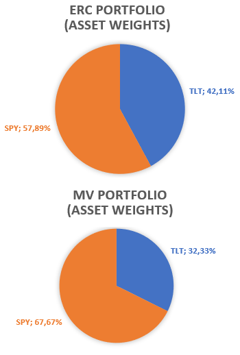
Something interesting to note in Figure 1 is that the ERC portfolio appears closer to an equally weighted portfolio than the MV portfolio, which is a general property discussed in Maillard et al.1.
Now, let’s suppose that the TLT ETF is somehow duplicated into a TLT’ ETF over the same period of time.
What would be the impact of this asset duplication on the above portfolios?
Answer is provided in Figure 2.
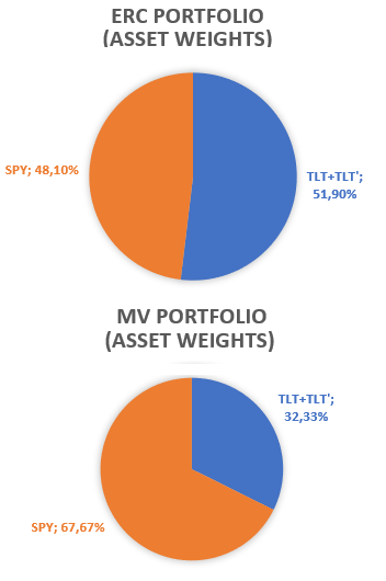
It is visible on Figure 2 that:
-
The weights of the ERC portfolio in the original assets are (severely) impacted by the duplication of TLT ETF.
The ERC portfolio is said be non duplication invariant.
-
The weights of the MV portfolio in the original assets are left unchanged7 by the duplication of the TLT ETF.
The MV portfolio is said to be duplication invariant.
This lack of duplication invariance means that ERC portfolios are generally biased toward assets with multiple representations2, so that the asset universe is an important factor when considering [ERC] portfolios8.
As an example, for a portfolio invested in bonds and equities, the number […] of bond versus equity will dramatically affect the risk contribution of the [ERC] portfolio from each category3.
Indeed, as detailed in Roncalli and Weisang8:
If the universe includes 5 equity indices and 5 bond indices, then the ERC portfolio will be well balanced between equity and bond in terms of risk. Conversely, if the universe includes 7 equity indices and 3 bond indices, the equity risk of the ERC portfolio represents then 70% of the portfolio’s total risk, a solution very unbalanced between equity and bond risks.
Figure 3 illustrates this imbalance within the SPY-TLT universe, with the TLT duplicated 5 times (resp. 3 times) and the SPY ETF duplicated 5 times (resp. 7 times).
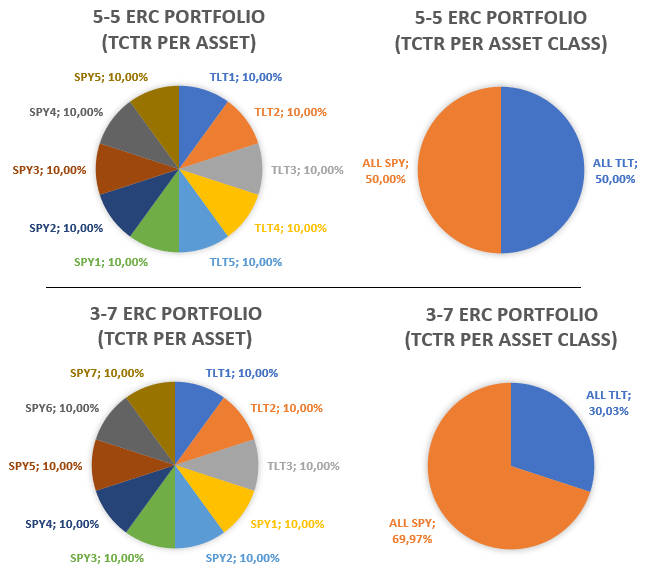
Interestingly, such a behavior is not in violation of the mathematical objective of the ERC portfolio9, but is nevertheless in clear violation of the ERC portfolio philosophy based on diversification1.
Notes:
- Asset weights in Figure 1 and Figure 2 might seem surprising at first sight (higher weights for the SPY ETF v.s. the TLT ETF), but 2023 has been a particular year for U.S. Treasuries… For reference, the exact (co)variances of the SPY and TLT ETFs are provided in Figure 5.
- For more discussion about duplication invariance, see for example Gava and Turc10, which introduces a quantitative measure of the sensitivity of a portfolio to duplication.
The cluster risk parity portfolio
Description
One possible solution to the problem of the sensitivity of the ERC portfolio discussed in the previous section is a careful selection of the universe of assets.
Another possible solution is to slightly alter the ERC portfolio construction process by taking into account both the asset and the asset class level, which is the solution proposed by Varadi3 and Kapler4 under the name cluster risk parity (CRP) portfolio.
In details, the CRP portfolio is computed through a three-step process, detailed below.
Notes:
- Another cluster risk parity portfolio is described in the Quantpedia series Introduction to Clustering Methods In Portfolio Management, but the two portfolio construction methodologies are not the same.
Step 1 - Partitioning the universe of assets into clusters
The first step consists in using a clustering algorithm to group similar assets together within the considered universe of assets.
This results in $k$ clusters11 $\mathcal{G}_1,…,\mathcal{G}_k$, $1 \leq k \leq n$, each corresponding to an asset class automatically determined by the clustering algorithm.
The purpose of this step is to avoid the need for artificial or manual grouping3 of the assets and enables the [CRP] portfolio to adapt to changes […] without having to run a lot of ad hoc analysis and having to make continual adjustments3.
Using the same hierarchical clustering algorithm as the one used in the Hierarchical Clustering-Based Risk Parity algorithm and using asset data over the period 03rd January 2023 - 29th December 20236, Figure 4 illustrates this first step for a universe of 10 ETFs representative12 of misc. asset classes:
- U.S. stocks (SPY ETF)
- European stocks (EZU ETF)
- Japanese stocks (EWJ ETF)
- Emerging markets stocks (EEM ETF)
- U.S. REITs (VNQ ETF)
- International REITs (RWX ETF)
- U.S. 7-10 year Treasuries (IEF ETF)
- U.S. 20+ year Treasuries (TLT ETF)
- Commodities (DBC ETF)
- Gold (GLD ETF)
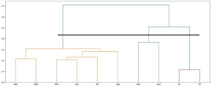
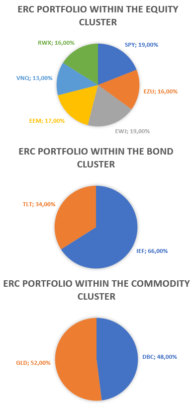
Figure 4 shows that 3 clusters/asset classes have been automatically determined by the hierarchical clustering algorithm over the studied period, materialized by the thick black dendrogram cut:
- An equity cluster $\mathcal{G}_1$ made of the equity ETFs SPY, EZU, EWJ, EEM and of the real estate ETFs VNQ, RWX
- A bond cluster $\mathcal{G}_2$ made of the bond ETFs IEF, TLT
- A commodity cluster $\mathcal{G}_3$ made of the commodity ETF DBC and of the gold ETF GLD
Step 2 - Assets weights computation within each cluster
The second step consists in computing the ERC portfolio within each cluster $\mathcal{G}_i$, $i=1..k$.
This results in $k$ vectors of asset weights $w_{i}^* \in [0,1]^{n}$, $i=1..k$.
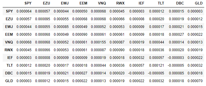
Using as input the covariance matrix $\Sigma$ provided in Figure 513, the ERC portfolio computed within each cluster $\mathcal{G}_1$, $\mathcal{G}_2$ and $\mathcal{G}_3$ defined in the previous sub-section is displayed in Figure 6.
Step 3 - Assets weights computation across all clusters and final assets weights computation
The third and last step consists in computing the ERC portfolio across all clusters $\mathcal{G}_i$, $i=1..k$.
For this:
-
Because the $k$ clusters $\mathcal{G}_1,…,\mathcal{G}_k$ correspond to $k$ risk factors, whose loadings matrix $A \in \mathcal{M}(\mathbb{R}^{n \times k})$ - in the original asset weights - is $ A = \begin{pmatrix} w_1^* & w_2^* & … & w_k^* \end{pmatrix} $, the cluster covariance matrix $\Sigma_c \in \mathcal{M}(\mathbb{R}^{k \times k})$ is equal14 to $ A^t \Sigma A $.
-
Thanks to that cluster covariance matrix, it is possible to compute the ERC portfolio across all clusters.
This results in a vector of cluster weights $w_c^* \in [0,1]^{k}$.
-
Then, all remaining is to convert the vector of cluster weights $w_c^*$ into the final vector of asset weights $w^* \in [0,1]^n$ through the formula $w^* = A w_c^*$.
Continuing the example from the previous sub-section:
-
The loading matrix $A$, deduced from Figure 6, is:
\[A = \begin{pmatrix} 0.19 & 0 & 0 \\ 0.16 & 0 & 0 \\ 0.19 & 0 & 0 \\ 0.17 & 0 & 0 \\ 0.13 & 0 & 0 \\ 0.16 & 0 & 0 \\ 0 & 0.66 & 0 \\ 0 & 0.34 & 0 \\ 0 & 0 & 0.48 \\ 0 & 0 & 0.52 \\ \end{pmatrix}\] -
The cluster covariance matrix $\Sigma_c$ is:
\[\Sigma_c = A^t \Sigma A = \begin{pmatrix} 0.000063 & 0.000014 & 0.000016 \\ 0.000014 & 0.000053 & 0.000011 \\ 0.000016 & 0.000011 & 0.000047 \\ \end{pmatrix}\] -
The vector of cluster weights of the across-cluster ERC portfolio is:
\[w_c^* = \begin{pmatrix} 0.30 \\ 0.34 \\ 0.36 \end{pmatrix}\] -
The vector of asset weights of the CRP portfolio, $w^* = A w_c^*$, is displayed in Figure 7:
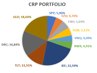
Figure 7. Example of CRP portfolio computation, final portfolio weights, 10-ETF universe.
Practical performances
The CRP portfolio has been empirically benchmarked against several other portfolios within different multi-asset classes universes415 and its performances, especially in terms of risk-adjusted returns, have been found to be excellent.
On this aspect, Varadi3 concludes that:
The [CRP portfolio] is perhaps the most robust method of passive portfolio allocation, and it also produces the best risk-adjusted returns without relying as much on the low-volatility factor or bond/fixed income performance.
Implementation in Portfolio Optimizer
Portfolio Optimizer allows to easily compute the CRP portfolio through the endpoint /portfolios/optimization/equal-risk-contributions/clustering-based, with optional support
for minimum and maximum asset weights constraints.
For maximum flexibility, the partitioning of the considered universe of assets into clusters is expected to be provided in input to that endpoint, which can be done using either:
- Any clustering algorithm available on the user side
- Any clustering algorithm provided by Portfolio Optimizer:
- The Fast Threshold Clustering Algorithm (FTCA), available through the endpoint
/assets/clustering/ftca - The hierarchical clustering algorithm used in the Hierarchical Clustering-Based Risk Parity algorithm, available through the endpoint
/assets/clustering/hierarchical
- The Fast Threshold Clustering Algorithm (FTCA), available through the endpoint
Conclusion
This concludes the description of the CRP portfolio, a little known but excellent framework to consider for a robust risk parity approach15.
As usual, feel free to connect with me on LinkedIn or to follow me on Twitter.
–
-
See Maillard, S., Roncalli, T., Teiletche, J.: The properties of equally weighted risk contribution portfolios. J. Portf. Manag. 36, 60–70 (2010). ↩ ↩2 ↩3 ↩4 ↩5 ↩6 ↩7 ↩8 ↩9 ↩10
-
See Choueifaty, Y., Tristan Froidure, T., Reynier, J. Properties of the Most Diversified Portfolio. Journal of Investment Strategies, Vol.2(2), Spring 2013, pp.49-70. ↩ ↩2 ↩3 ↩4
-
See David Varadi, CSSA, Cluster Risk Parity and David Varadi, CSSA, Cluster Risk Parity (CRP) versus Risk Parity (RP) and Equal Risk Contribution (ERC). ↩ ↩2 ↩3 ↩4 ↩5 ↩6
-
See Michael Kapler, Systematic Investor Blog, Cluster Portfolio Allocation and Michael Kapler, Systematic Investor Blog, Cluster Risk Parity back-test. ↩ ↩2 ↩3
-
When the risk measure is defined as the portfolio volatility; other risk measures can be used instead, c.f. Maillard et al.1. ↩
-
(Adjusted) prices have have been retrieved using Tiingo. ↩ ↩2
-
This property is established in all generality in Maillard et al.1. ↩
-
See Roncalli, Thierry and Weisang, Guillaume, Risk Parity Portfolios with Risk Factors and Roncalli & G. Weisang, Risk parity portfolios with risk factors, Quantitative Finance. ↩ ↩2
-
Per construction of the ERC portfolio, ll assets present in that portfolio are guaranteed to have the same total risk contributions. ↩
-
See Gava J, Turc J. The Properties of Alpha Risk Parity Portfolios. Entropy. 2022; 24(11):1631. ↩
-
Assumed to form a partition of the universe of assets. ↩
-
These ETFs are used in the Adaptative Asset Allocation strategy from ReSolve Asset Management, described in the paper Adaptive Asset Allocation: A Primer16. ↩
-
This covariance matrix is the empirical asset covariance matrix computed from the arithmetic returns of the 10 assets over the period 04th January 2023 - 29th December 2023. ↩
-
This is a direct application of the formula for the covariance matrix of a linear transformation of a random vector, c.f. for example Wikipedia, Covariance matrix. ↩
-
See ReSolve Asset Management, Dynamic asset allocation for practitioners part 5: robust risk parity. ↩ ↩2
-
See Butler, Adam and Philbrick, Mike and Gordillo, Rodrigo and Varadi, David, Adaptive Asset Allocation: A Primer. ↩